Update 5/17: As discussed in the comments, the reason the results are so exaggerated is because it is missing portfolio rebalancing to account for the changing hedge ratio. It would be interesting to try an adaptive hedge ratio that requires only weekly or monthly rebalancing to see how legitimately profitable this type of strategy could be.
Welcome back! This week’s post will backtest a basic mean reverting strategy on a cointegrated ETF pair time series constructed using the methods described in part I. Since the EWA (Australia) – EWC (Canada) pair was found to be more naturally cointegrated, I decided to run the rolling linear regression model (EWA chosen as the dependent variable) with a lookback window of 21 days on this pair to create the spread below.
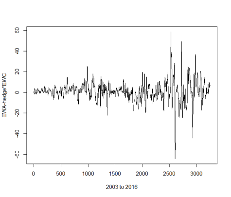
With the adaptive hedge ratio, the spread looks well suited to backtest a mean reverting strategy on. Before that, we should check what the minimum capital required to trade this spread is. Though everyone has a different margin requirement, I thought it would be useful to walkthrough how you would calculate the capital required. In this example we assume our broker allows a margin of 50%. We first will compute the daily ratio between the pair, EWC/EWA. This ratio represents the amount of EWA shares for each share of EWC that must be owned to have an equal dollar move for every 1% move. The ratio fluctuates daily but has a mean of 1.43. This makes sense because EWC, on average, trades at higher price. We then multiply these ratios by the rolling beta. Then for reference, we can fix the held EWC shares to 100 and multiply the previous values (ratios*rolling beta) by 100 to determine the amount of EWA shares that would be held. The amount of capital required to hold this spread can then be calculated with the equation: margin*abs((EWC price * 100) + (EWA price * calculated shares)). This is plotted for our example below.
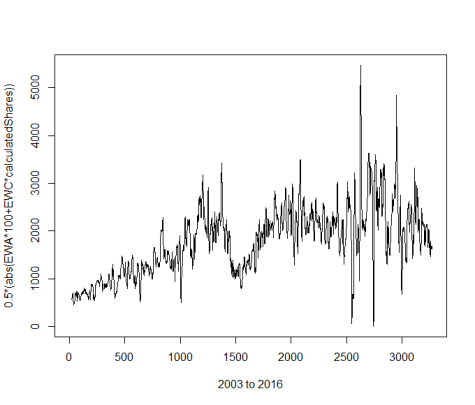
From this plot we can see that the series has a max value of $5,466 which is not a relatively large required capital. I hypothesize that the less cointegrated a pair is, the higher the minimum capital will be (try the EWZ-IGE pair).
We can now go ahead and backtest the figure 1 time series! A common mean reversal strategy uses Bollinger Bands, where we enter positions when the price deviates past a Z-score/standard deviation threshold from the mean. The exit signals can be determined from the half-life of its mean reversion or it can be based on the Z-score. To avoid look-ahead bias, I calculated the mean, standard deviation, and Z-score with a rolling 50-day window. Unfortunately, this window had to be chosen with data-snooping bias but was a reasonable choice. This backtest will also ignore transaction costs and other spread execution nuances but should still reasonably reflect the strategy’s potential performance. I decided on the following signals:
- Enter Long/Close Short: Z-Score < -1
- Close Long/Enter Short: Z-Score > 1
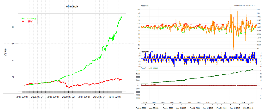
This is a standard Bollinger Bands strategy and results were encouraging.
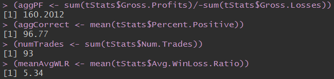
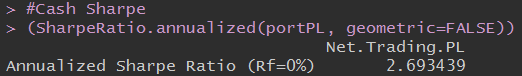
Though it made a relatively small amount of trades over 13 years, it boasts an impressive 2.7 Sharpe Ratio with 97% positive trades. Below on the left we can see the strategy’s performance vs. SPY (using very minimal leverage) and on the right the positions/trades are shown.
Overall, this definitely supports the potential of trading cointegrated ETF pairs with Bollinger Bands. I think it would be interesting to explore a form of position sizing based on either market volatility or the correlation between the ETF pair and another symbol/ETF. This concludes my analysis of cointegrated ETF pairs for now.
Acknowledgments: Thank you to Brian Peterson and Ernest Chan for explaining how to calculate the minimum capital required to trade a spread. Additionally, all of my blog posts have been edited prior to being published by Karin Muggli, so a huge thank you to her!
Note: I’m currently looking for a full-time quantitative research/trading position beginning summer/fall 2017. I’m currently a senior at the University of Washington, majoring in Industrial and Systems Engineering and minoring in Applied Mathematics. I also have taken upper level computer science classes and am proficient in a variety of programming languages. Resume: https://www.pdf-archive.com/2017/01/31/coltonsmith-resume-g/. LinkedIn: https://www.linkedin.com/in/coltonfsmith. Please let me know of any open positions that would be a good fit for me. Thanks!
Full Code:
detach("package:dplyr", unload=TRUE)
require(quantstrat)
require(IKTrading)
require(DSTrading)
require(knitr)
require(PerformanceAnalytics)
require(quantstrat)
require(tseries)
require(roll)
require(ggplot2)

# Full test
initDate="1990-01-01"
from="2003-01-01"
to="2015-12-31"

## Create "symbols" for Quanstrat
## adj1 = EWA (Australia), adj2 = EWC (Canada)

## Get data
getSymbols("EWA", from=from, to=to)
getSymbols("EWC", from=from, to=to)
dates = index(EWA)

adj1 = unclass(EWA$EWA.Adjusted)
adj2 = unclass(EWC$EWC.Adjusted)

## Ratio (EWC/EWA)
ratio = adj2/adj1

## Rolling regression
window = 21
lm = roll_lm(adj2,adj1,window)

## Plot beta
rollingbeta <- fortify.zoo(lm$coefficients[,2],melt=TRUE)
ggplot(rollingbeta, ylab="beta", xlab="time") + geom_line(aes(x=Index,y=Value)) + theme_bw()

## Calculate the spread
sprd <- vector(length=3273-21)
for (i in 21:3273) {
sprd[i-21] = (adj1[i]-rollingbeta[i,3]*adj2[i]) + 98.86608 ## Make the mean 100
}
plot(sprd, type="l", xlab="2003 to 2016", ylab="EWA-hedge*EWC")

## Find minimum capital
hedgeRatio = ratio*rollingbeta$Value*100
spreadPrice = 0.5*abs(adj2*100+adj1*hedgeRatio)
plot(spreadPrice, type="l", xlab="2003 to 2016", ylab="0.5*(abs(EWA*100+EWC*calculatedShares))")

## Combine columns and turn into xts
close = sprd
date = as.data.frame(dates[22:3273])
data = cbind(date, close)
dfdata = as.data.frame(data)
xtsData = xts(dfdata, order.by=as.Date(dfdata$date))
xtsData$close = as.numeric(xtsData$close)
xtsData$dum = vector(length = 3252)
xtsData$dum = NULL
xtsData$dates.22.3273. = NULL

## Add SMA, moving stdev, and z-score
rollz<-function(x,n){
avg=rollapply(x, n, mean)
std=rollapply(x, n, sd)
z=(x-avg)/std
return(z)
}

## Varying the lookback has a large affect on the data
xtsData$zScore = rollz(xtsData,50)
symbols = 'xtsData'

## Backtest
currency('USD')
Sys.setenv(TZ="UTC")
stock(symbols, currency="USD", multiplier=1)

#trade sizing and initial equity settings
tradeSize <- 10000
initEq <- tradeSize

strategy.st <- portfolio.st <- account.st <- "EWA_EWC"
rm.strat(portfolio.st)
rm.strat(strategy.st)
initPortf(portfolio.st, symbols=symbols, initDate=initDate, currency='USD')
initAcct(account.st, portfolios=portfolio.st, initDate=initDate, currency='USD',initEq=initEq)
initOrders(portfolio.st, initDate=initDate)
strategy(strategy.st, store=TRUE)

#SIGNALS
add.signal(strategy = strategy.st,
name="sigFormula",
arguments = list(label = "enterLong",
formula = "zScore < -1", cross = TRUE), label = "enterLong") add.signal(strategy = strategy.st, name="sigFormula", arguments = list(label = "exitLong", formula = "zScore > 1",
cross = TRUE),
label = "exitLong")

add.signal(strategy = strategy.st,
name="sigFormula",
arguments = list(label = "enterShort",
formula = "zScore > 1",
cross = TRUE),
label = "enterShort")

add.signal(strategy = strategy.st,
name="sigFormula",
arguments = list(label = "exitShort",
formula = "zScore < -1",
cross = TRUE),
label = "exitShort")

#RULES
add.rule(strategy = strategy.st,
name = "ruleSignal",
arguments = list(sigcol = "enterLong",
sigval = TRUE,
orderqty = 15,
ordertype = "market",
orderside = "long",
replace = FALSE,
threshold = NULL),
type = "enter")

add.rule(strategy = strategy.st,
name = "ruleSignal",
arguments = list(sigcol = "exitLong",
sigval = TRUE,
orderqty = "all",
ordertype = "market",
orderside = "long",
replace = FALSE,
threshold = NULL),
type = "exit")

add.rule(strategy = strategy.st,
name = "ruleSignal",
arguments = list(sigcol = "enterShort",
sigval = TRUE,
orderqty = -15,
ordertype = "market",
orderside = "short",
replace = FALSE,
threshold = NULL),
type = "enter")

add.rule(strategy = strategy.st,
name = "ruleSignal",
arguments = list(sigcol = "exitShort",
sigval = TRUE,
orderqty = "all",
ordertype = "market",
orderside = "short",
replace = FALSE,
threshold = NULL),
type = "exit")

#apply strategy
t1 <- Sys.time()
out <- applyStrategy(strategy=strategy.st,portfolios=portfolio.st)
t2 <- Sys.time()
print(t2-t1)

#set up analytics
updatePortf(portfolio.st)
dateRange <- time(getPortfolio(portfolio.st)$summary)[-1]
updateAcct(portfolio.st,dateRange)
updateEndEq(account.st)

#Stats
tStats <- tradeStats(Portfolios = portfolio.st, use="trades", inclZeroDays=FALSE)
tStats[,4:ncol(tStats)] <- round(tStats[,4:ncol(tStats)], 2)
print(data.frame(t(tStats[,-c(1,2)])))

#Averages
(aggPF <- sum(tStats$Gross.Profits)/-sum(tStats$Gross.Losses))
(aggCorrect <- mean(tStats$Percent.Positive))
(numTrades <- sum(tStats$Num.Trades))
(meanAvgWLR <- mean(tStats$Avg.WinLoss.Ratio))

#portfolio cash PL
portPL <- .blotter$portfolio.EWA_EWC$summary$Net.Trading.PL

## Sharpe Ratio
(SharpeRatio.annualized(portPL, geometric=FALSE))

## Performance vs. SPY
instRets <- PortfReturns(account.st)
portfRets <- xts(rowMeans(instRets)*ncol(instRets), order.by=index(instRets))

cumPortfRets <- cumprod(1+portfRets)
firstNonZeroDay <- index(portfRets)[min(which(portfRets!=0))]
getSymbols("SPY", from=firstNonZeroDay, to="2015-12-31")
SPYrets <- diff(log(Cl(SPY)))[-1]
cumSPYrets <- cumprod(1+SPYrets)
comparison <- cbind(cumPortfRets, cumSPYrets)
colnames(comparison) <- c("strategy", "SPY")
chart.TimeSeries(comparison, legend.loc = "topleft", colorset = c("green","red"))

## Chart Position
rets <- PortfReturns(Account = account.st)
rownames(rets) <- NULL
charts.PerformanceSummary(rets, colorset = bluefocus)

Hello,
Why the code isn’t rigth formated ? t1 <- Sys.time()
but nice article !!
Regards
Ludo.
LikeLike
Fixed. For some reason it didn’t render the equality signs correctly. Thanks for catching that!
LikeLike
First of all, Thank you for a wonderful article. I have tested the code with CVX/XOM and GLD/SLV pairs. In both cases the returns are astronomical. This makes me a bit suspicious about the code that either there is some look ahead bias or the calculations are not correct somewhere. I will spend sometime over the weekend to see if I can find anything.
But the theory and the application are very helpful. Thanks.
LikeLike
Hi, assuming you constructed those spreads correctly, I think the returns are largely inflated due to ignoring all the nuances in actually executing a pair trading strategy like this. I don’t believe there is any look-ahead bias or incorrect calculations. Looking at the spread’s time series, it makes sense that any reasonable mean reversion strategy should have astronomical returns with very few losing trades but if you were to actually implement this strategy then there would be other things that you would have to take into account. I’m not sure how much this would affect the backtest results but for this post I merely wanted to explore its potential.
Thanks for reading!
LikeLike
Understood and thanks for your kind response. One other quick question. Where does the 98.86608 come from to make the mean 100? I am working on replicating this using my own framework to see what the results would look like. I should have an answer shortly. Thanks.
LikeLike
I just did 100-mean(EWA-hedge*EWC) to get that. It doesn’t matter what the mean of the time series is so I just made it 100 for easier numbers.
LikeLike
Hi there, nice post , again!
Did you by any chance , calculate the half life using the O-U Equation , or the in-sample-average-time(days)-in-trade-until-mean-reversion? If you did, what was it ?
also, i dont know if I read it right from the start, but, did you trade on the same period that you used to test for cointegration ? (in sample)
or, did you use a rolling 21 days window for the moving hedge ratio between the pairs components while testing them for cointegrationinside this moving window and them filtering trades for both one of the triggers + cointegration at that time ?
tanks again.
best regards!
LikeLike
Hey,
I did not calculate the half-life for this EWA-EWC series but in the last post my code to do so with the O-U equation is included if you want to!
I constructed the series using the rolling 21 day window for the hedge ratio as explained in part I. I then added the the rolling Z-Score indicator using a 50 day window (this was chosen arbitrarily with data snooping bias).
If I understand your question correctly, this should be functionally the same as calculating the hedge ratio and the Z-Score indicator at the same time.
Thanks for reading!
LikeLike
Hi there,
Yeah, what I meant to ask was if you realized that you used the same in sample data, the same data where you tested the pair for cointegration, both for testing for cointegration + calculating the rolling 50 day statistics + calculating the rolling 21 day hedge ratio (beta) and trading.
I didn’t have the time to run your script, yet, and debug it properly, so excuse me if that’s clear in the code and I’m making a redundant comment.
Thanks
LikeLike
Yes, I create the series with the rolling 21 day hedge ratio and then calculated the rolling 50 day statistics from this series while trading it.
I used these rolling windows to prevent any look-ahead bias. Is there a flaw in this? I don’t know what would be out of sample data for this example.
Thanks!
LikeLike
Well, as long as you are not trading the pair because it showed to be cointegrated on the same period that you are using for trading, it’s OK. (IF and only IF you are trading the pair BECAUSE of the cointegration, and wouldn’t do it otherwise).
I’ll try to explain it better below :
Using a 21 days moving window for calculating the hedge ratio, a 50 days moving window for the BBs parameters, and assuming that you are using a one year (say 252 days) look back window for cointegration testing (I think I recall that Dr. Chan preferred at least 3yrs for this?).
So, in the first 21 days you calculate the first moving hedge ratio for the 22nd day, and update it daily. Your first data point will be at T+22.
Now that you have the necessary information for creating the mean reverting spread (prices of each ETF and the hedge ratio) you can start populating this new vector and, after 50 data points you will have the first data points for the mean and stdv of the spread (y-hedge ratio *x). So, now we’re at the 22nd + 50 = 72nd day for the first data point of the spread + BBs.
OK, so far so good.
Now we can start trading the pair…
UNLESS you still have to test it for cointegration.
If you do test it for cointegration and require it to be true for trading the pair, then your first data point for out of sample testing would be 22+252. From the first available point of the spread using the 21 days hedge ratio (22nd day) to one year after that (252 days), so your first out of sample data point would be @ day 274 onward, only taking trades if both the cointegration vector (imagine a binary vector where 1==cointegrated and 0==nope) shows 1 and one of the trigger points is hit by the spread (1 stdv as you said).
That’s it!
PS: again, if that is already clear in the code, I’m sorry cause I haven’t been able to run it yet. I’ve been reading and posting from my cellphone.
LikeLike
Ah okay, I understand what you are saying. I guess the strategy is based on the assumption that using an 21 day adaptive hedge ratio creates a sufficiently stationary series on a pair that is believed to be somewhat cointegrated. For example, in part I, the EWZ-IGE pair is much less cointegrated but with an adaptive hedge ratio produces a stationary series. This series is not as nice as the EWA-EWC pair so I would assume that in this case the strategy would not perform as well on the EWZ-IGE pair.
LikeLike
Thanks for the reply.
Are you sure there is no look ahead bias within the backtesting framework (I never used any if those packages) and the RollZ function for calculating the 50 days parameters in the spread series? It seems that the trading strategy core uses InitDate as the starting point for the test, and that would be before any of the calculations on the series and spread were made.
I’m asking because of the stellar results. When the results are too good to be true, they normally are not true, even though you don’t account for slippage, liquidity, signal generation, costs, etc.
I hope I’m wrong!
Best
LikeLike
Run my code and then view the mktdata object. This shows when the indicators and signals are calculated. You’re correct, it isn’t able to start trading the strategy until awhile after the InitDate and mktdata shows this.
Someone else also questioned look-ahead bias but we were both unable to find any. Like I said, looking at the constructed time series, the returns should be incredible for any adequate mean reversion strategy. I personally don’t know the feasibility of actually trading this constructed series though. Let me know if you do have any ideas where look-ahead bias was introduced!
Thanks
LikeLike
I just ran all of your code , exported the dataframes and etcs to CSV and reviewed it in Excel, and indeed, it is right! there are some differences between the calculations, but that must be because of the regression methods in R and Excel, etc..
I took a heavy beating from those R trading packages that i had never used. I tried to insert an 1 day delay for the trades, but couldn’t..
the series start @ “2003-01-01”, so the 1st one month is taken off by the calculation of the moving hedge ratio of 21 days. after that there is the 50 days calculation of the mean/stdv moving window, and only after that that the spread starts to exist.
One interesting point is that the strategy keeps scaling in when the spread is still outside the triggers, right ? so sometimes there are 3..4.. positions at the same time, pyramiding the trades.
if you could share some links about the packages so one can understand their logic, id be very glad!
best regards
LikeLike
Hi,
I am trying to duplicate this algorithm with python and can’t get this stellar returns. I have some doubt about how I calculate rolling beta with this code :
rolling_beta = statsmodels.api.OLS(price1, price2).fit().params[1]
Do you think I missed something with OLS function ?
Thanks
LikeLike
Colton, I think I may have figured out why the results are so good on paper but in reality this may not translate to real money trading this strategy…I may be completely off but I am still trying to make sense of the results.
I have confirmed that there is no look ahead bias, So that’s not an issue.
Let’s look at a sample transaction to show where the issue is.
On “3/6/2017” the strategy opens a short position of -15 shares @ $110.5143 for a total of (-$1657.7145).
This position is closed on “4/5/2017” @ $89.3274 for a total of $1339.911
This transaction on paper made a Profit of $317.8035.
All good so far. Now lest see what happens in the trading account to trade this position.
On “3/6/2017”
EWA is @ $21.92 and EWC is @ $26.88. To initiate a short position you would have to
sell 47 shares of EWA & Buy 100 shares of EWC
This transaction translates to 47 x $21.92 =1030.24 for EWA and 100 x 26.88 = $2688 for EWC.
On “4/5/2017” when the strategy closes the position, EWA is trading @ $22.45 and EWC is trading @ $26.77
This trade would have resulted in a Loss of $35.91 instead of a gain of $317.8035
The reason why the strategy makes money on paper is because the Synthetic Spread value shrunk because the Beta value changed not because the prices have changed in the right direction.
Hope I didn;t make any mistake here but happy to provide any additional details. I am happy to stand corrected and make money like the strategy does on paper 🙂
Thanks.
LikeLike
This strategy is missing any portfolio rebalancing. If the optimal hedge ratio according to the lookback n is recalculated every day then any open positions need to be rebalanced periodically to ensure that it is as close to the hedged spread as possible. In the code above I can see that the code is using the dynamically hedged spread as the price of the “portfolio” and buys and sells this according to the z-score signals. However, as the comment above by Quant Trader highlights, the profits will be greatly exaggerated due to the changes in the synthetic spread caused by the changing hedged ratio.
Please let me know what you think?
LikeLike
Yes, Quant Trader and V-Man you are correct. This is missing portfolio rebalancing. It would be interesting to try a less frequent rebalancing/adaptive hedge ratio to see how legitimately profitable this type of strategy could be. Thanks for your exploration!
LikeLike
Very interesting article! Will you write another post testing different rebalancing periods?
Thanks
LikeLike
Hi Colton,
Neat article, thanks for sharing. I’m an old-school CS major looking at quant trading. What language are you using in the code example provided in this post?
LikeLike
Hi Nathan,
The code is R. There are similar packages in Python as well.
LikeLike