Risk-Neutral Probability Distributions: CLK2020

Colton Smith & Kevin Schneider

Risk-neutral probability distributions (RND) are used to compute the fair value of an asset as a discounted conditional expectation of its future payoff. In 1978, Breeden and Litzenberger presented a method to derive this distribution for an underlying asset from observable option prices [1]. The derivation of the relationship is well presented in A Simple and Reliable Way to Compute Option-Based Risk-Neutral Distributions by Allan Malz which is summarized below [2].

In the absence of arbitrage, the European call option value can be related to the discounted expected terminal value under the risk-neutral distribution.

$c(t, K, \tau) = e^{-r_t \tau} \tilde{\mathbb{E}}_t\left[\max(S_T - K, 0)\right] = e^{-r_t \tau} \int_K^\infty (s-K) \tilde{\pi}_t(s) ds$

where

$\begin{aligned} t &= \text{Time of call option value observation} \\ T &= \text{Expiration} \\ \tau &= \text{Time till expiration in years (} T-t \text{)} \\ K &= \text{Strike price} \\ S_T &= \text{Underlying price at expiration} \\ S_t &= \text{Time-}t \text{ underlying price} \\ r_t &= \text{Time-}t \text{ risk-free interest rate} \\ \tilde{\mathbb{E}}_t[\cdot] &= \text{The expectation from the risk-neutral probability distribution taken at time-}t \\ \tilde{\pi}_t(\cdot) &= \text{The risk-neutral probability density function of }S_T\text{ at time-}t \end{aligned}$

Differentiating the call option value with respect to the strike price gives what Malz refers to as the “exercise-price delta”.

$\frac{\partial}{\partial K}c(t, K, \tau) = e^{-r_t \tau}\left[\int_0^K \tilde{\pi}_t(s) ds - 1\right]$

This result contains the risk-neutral cumulative distribution function $\tilde{\Pi}_t(K)$ , the probability that the underlying price at expiration will be $K$ or lower.

$\tilde{\Pi}_t(K) = \int_0^K \tilde{\pi}_t(s) ds = 1 + e^{r_t \tau}\frac{\partial}{\partial K}c(t, K, \tau)$

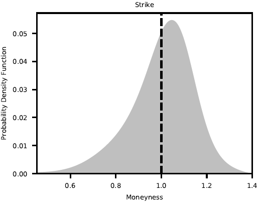
To arrive at the risk-neutral probability density function, one more derivative with respect to the strike price is needed.

$\tilde{\pi}_t(K) = e^{r_t \tau}\frac{\partial^2}{\partial K^2}c(t, K, \tau)$

Now we will present an overview of deriving these distributions numerically using the infamous May 2020 WTI Crude Oil contract that went negative in April. Albeit these are American options, the analysis is interesting nonetheless.

To approximate the partial derivatives, we need option prices for a fine grid of strike prices. In fact, Breeden and Litzenberger simply assume that options are traded at every positive strike price. The first step is thus to fit a smooth function to the Black-Scholes implied volatility smile of the option prices. We interpolate implied volatilities rather than prices because the former tend to be smoother and better behaved. To ensure that the prices and implied volatilities are clean, open interest can be used to weight or exclude certain strikes. We constructed the smile using out-of-the-money calls and puts as these options tend to have more open interest than their in-the-money equivalents. Numpy’s polyfit is then used to interpolate and extrapolate the smile as needed.

Implied_Vol_Fit

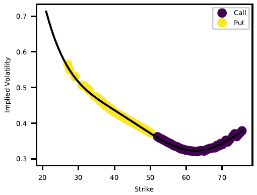
The second step is to calculate the call prices using the Black-Scholes formula for constant rates with your fitted implied volatility function, underlying price, time to expiration, and observed risk-free rate.

Call_Prices

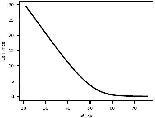
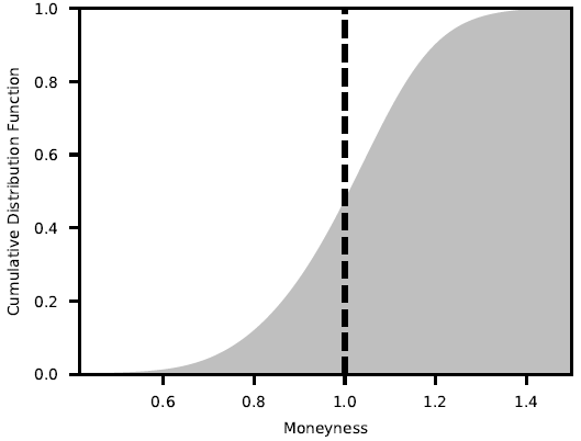
The third step, following the mathematical derivation above, is to calculate $\tilde{\Pi}_t(K)$ using the first derivative of the call price with respect to the strike price. Numpy’s diff function will numerically difference your call price function. This effectively corresponds to using a forward difference to approximate the partial derivative.

Cumulative_Distribution

To compare these distributions across strike prices, using moneyness, $\frac{K}{S_t}$ , as the x-axis is helpful. The fourth and final step, is to calculate $\tilde{\pi}_t(K)$ using the second derivative of the call price with respect to the strike price and scaling it by $e^{r_t\tau}$ .

Density_Function

It can be difficult to generate clean RNDs and through this process it became clear how cumbersome it would be to generate these over an extended time series. To evaluate the quality of the fit, we need to check a few conditions.

– The cumulative distribution needs to be bounded between 0 and 1
– The probability density function needs to integrate to 1 and remain positive
– The exercise-price delta needs to be monotone and bounded by $-e^{-r_t\tau}$ and 0
– The strike weighted probability density function needs to integrate to the underlying futures price

There are additional arbitrage conditions to consider on the fitted implied volatility smile but our distributions meet the above conditions nicely so will be sufficient for our analysis. In fact, the absence of arbitrage is one of the few assumptions needed for the above mathematical derivation to hold. Further implicit assumptions include constant interest rates, that the call option price is twice differentiable and that a (smooth) probability density function of the price of the underlying asset exists to start with. Importantly, there are no further restrictions on the probabilistic nature of the underlying asset price process.

The above technique was repeated on the CLK2020 option chain for the four dates shown in the figure below to see how the option implied volatility RNDs reacted to the developing macro landscape including Covid-19, OPEC+, and crude oil physical storage capacity. The analysis was not extended into April as the possibility of negative prices violate some of the fundamental assumptions used.

Futures_Price

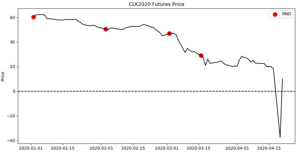
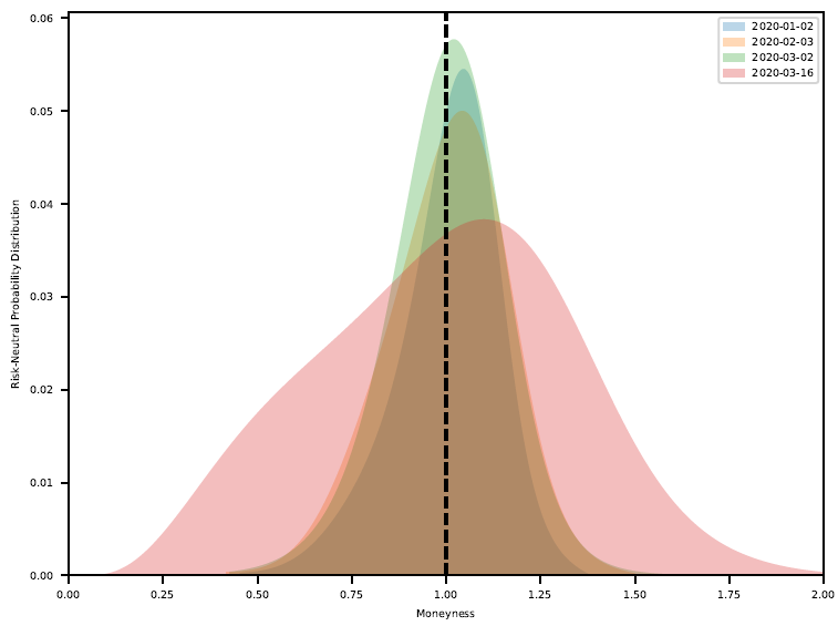
The resulting risk-neutral densities below tell quite the colorful story. In January, the distribution has a slight negative skew but high kurtosis. In February and March, the tail risk begins to emerge as the kurtosis decreases. Finally in mid-March the distribution flattens, presenting a very expressive RND.

Dist_Time_Series

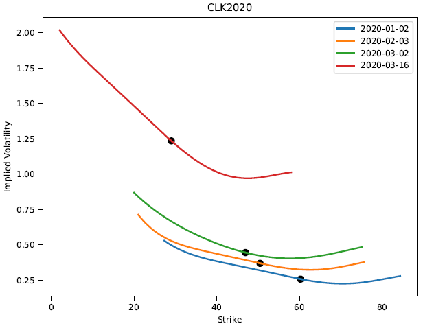
The corresponding fitted implied volatility smiles are shown below.

IV_Fits

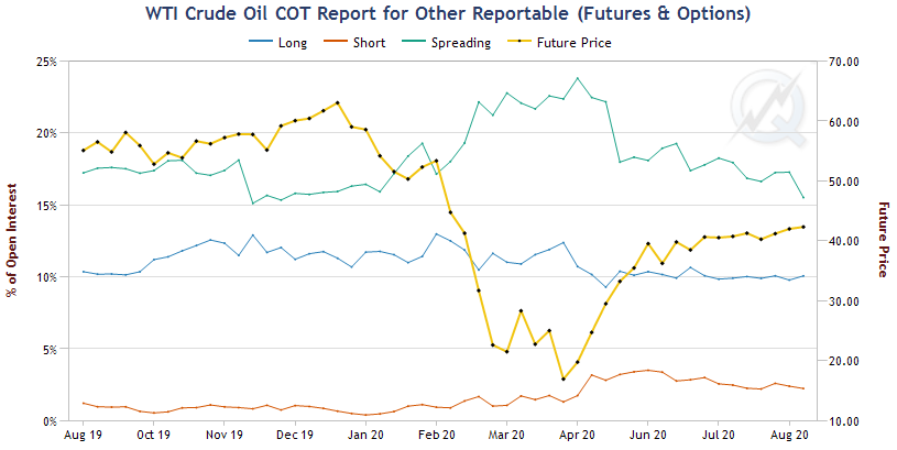
At the time, all eyes were on the calendar spreads and bear spreading the futures, short a nearby contract expiration month and long a deferred contact expiration month, was a popular trade. Based on the RND, this trade made sense if you believed that the bulk of the tail risk was in the nearby contract. Using the QuikStrike Commitment of Traders tool on the CME website we can look at the positioning of traders through this event [3]. The plots below show the positioning of the two groups that make up the “Non-Commercial” group of traders which includes hedge funds and large speculators.

COT_Managed_Money

COT_Other_Reportable

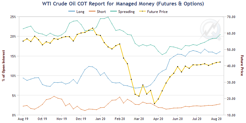
The “Managed Money” began the year with a larger spreading position (likely bear?) which decreased into February as a more concentrated short position grew. In April and May, they capitalized on the series of events, quickly building a fervent long position to ride the rally back up.

The “Other Reportables” held a large spreading positioning from the end of February until May, likely capturing the historical calendar spread move nicely.

It is important to emphasize that risk-neutral distributions are different from the real-world distributions which govern the likelihood of events in financial markets. A RND is an artificial probability distribution which allows the computation of option prices without specifying the risk aversion of investors (this insight is the reason for Scholes’ and Merton’s Nobel Prize in 1997). Thus, they are a very convenient mathematical tool but not a description of the real world.

Intuitively, RNDs merge real-world probabilities with investor’s attitudes toward risk. They tend to inflate the probability of economically bad states (which are rare but investors are very fearful of them) and understate the probability of booms. Hence, RNDs tend to be more negatively skewed than real-world distributions are.

In fact, the above idea can be formulated more rigorously. Let’s use a discrete setting for simplicity. Suppose we want to price an asset which generates a random cash flow of $X$ tomorrow (e.g. payoff of a call option). Finance theory suggests that today’s price, $c$ , should equal

$c = \mathbb{E}[XM],$

where the random variable $M$ takes the associated risk into account. Riskier payoffs should yield lower prices. $M$ is called the stochastic discount factor. In a discrete setting, the expectation is just the sum of outcomes weighted by the corresponding probabilities. Thus,

$\begin{aligned} c&=\sum_i x_i M_i p_i \\ &= \frac{1}{1+r} \sum_i x_iq_i \\ &= \frac{1}{1+r} \tilde{E}[X], \end{aligned}$

where $q_i = \frac{M_ip_i}{\sum M_ip_i}$ . Hence, $\sum q_i=1$ and $q_i\in[0,1]$ making them valid pseudo-(risk-neutral)-probabilities. Furthermore, denoting the risk-free rate by $r$ , and because $1=\sum (1+r) M_i p_i$ , we have $\frac{1}{\sum M_ip_i}=1+r$ , explaining the second equality. The final line is simply the discrete analogue to the equation at the beginning of this blog post: prices are discounted risk-neutral expectations of future payoffs.

This short derivation illustrates how merging the risk aversion (in form of $M$ ) and the real life probabilities ( $p$ ) yield the risk-neutral probabilities ( $q$ ). This however distorts and dilutes the probabilities. We can recover the risk-neutral probabilities $q$ from option prices, but this does not tell us what the real probabilities $p$ are because we do not know the right stochastic discount factor.

Changes in the RND can be attributed to changes in investor’s preferences, real-world probabilities, or both. A priori, it is impossible to know which of the three cases is true. Disentangling real-world probabilities from risk aversion typically requires a general equilibrium model of the economy and remains an open question for current research, see Ross (2015) [4] for a recent attempt.

References

[1] https://papers.ssrn.com/sol3/papers.cfm?abstract_id=2642349

[2] https://www.newyorkfed.org/medialibrary/media/research/staff_reports/sr677.pdf

[3] https://www.cmegroup.com/tools-information/quikstrike/commitment-of-traders-energy.html

[4] https://onlinelibrary.wiley.com/doi/abs/10.1111/jofi.12092

6 thoughts on “Risk-Neutral Probability Distributions: CLK2020”

Pingback: Quantocracy's Daily Wrap for 08/24/2020 | Quantocracy
Elie Mekanna says:

February 4, 2021 at 10:59 pm

Hi Colton,

Great article! Would it be possible to find the Python code used somewhere?

Thanks,

Elie

LikeLike

cfsmith says:

February 5, 2021 at 9:55 am

Hey Elie,

I don’t have the code available for this post because it’s very dependent on the structure of your input data and fit preferences. If a step in the process is unclear, shoot me an email and I’ll be happy to help.

Best,
Colton

LikeLike

Elie says:

February 14, 2021 at 10:50 pm

Hi Colton,

Thank you, I wrote up the code and got to the desired result. Only thing is that with polyfit it is not always the case that the fit is no-arbitrage.

Best,
Elie

LikeLike

1. dmhulme says:
  
  May 3, 2021 at 5:19 pm
  
  Hi Elie,
  
  Would you mind sharing the code that got you to the desired result? I am having trouble…
  
  Thanks,
  
  David
  
  LikeLike
  
David says:

May 3, 2021 at 4:47 pm

Hi Elie,

Would you mind sharing the code?

Thanks!

David

LikeLike