Update 5/17: As discussed in the comments, the reason the results are so exaggerated is because it is missing portfolio rebalancing to account for the changing hedge ratio. It would be interesting to try an adaptive hedge ratio that requires only weekly or monthly rebalancing to see how legitimately profitable this type of strategy could be.

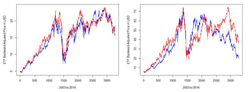
Welcome back! This week’s post will backtest a basic mean reverting strategy on a cointegrated ETF pair time series constructed using the methods described in part I. Since the EWA (Australia) – EWC (Canada) pair was found to be more naturally cointegrated, I decided to run the rolling linear regression model (EWA chosen as the dependent variable) with a lookback window of 21 days on this pair to create the spread below.

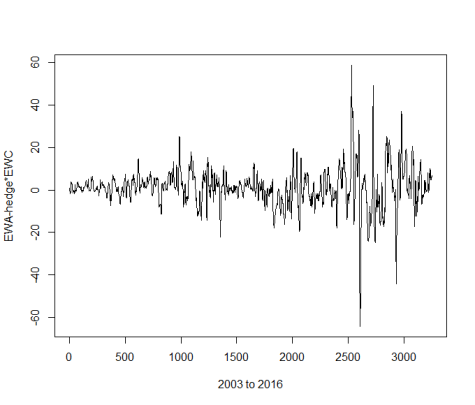
With the adaptive hedge ratio, the spread looks well suited to backtest a mean reverting strategy on. Before that, we should check what the minimum capital required to trade this spread is. Though everyone has a different margin requirement, I thought it would be useful to walkthrough how you would calculate the capital required. In this example we assume our broker allows a margin of 50%. We first will compute the daily ratio between the pair, EWC/EWA. This ratio represents the amount of EWA shares for each share of EWC that must be owned to have an equal dollar move for every 1% move. The ratio fluctuates daily but has a mean of 1.43. This makes sense because EWC, on average, trades at higher price. We then multiply these ratios by the rolling beta. Then for reference, we can fix the held EWC shares to 100 and multiply the previous values (ratios*rolling beta) by 100 to determine the amount of EWA shares that would be held. The amount of capital required to hold this spread can then be calculated with the equation: margin*abs((EWC price * 100) + (EWA price * calculated shares)). This is plotted for our example below.

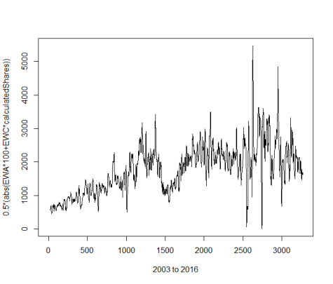
From this plot we can see that the series has a max value of $5,466 which is not a relatively large required capital. I hypothesize that the less cointegrated a pair is, the higher the minimum capital will be (try the EWZ-IGE pair).

We can now go ahead and backtest the figure 1 time series! A common mean reversal strategy uses Bollinger Bands, where we enter positions when the price deviates past a Z-score/standard deviation threshold from the mean. The exit signals can be determined from the half-life of its mean reversion or it can be based on the Z-score. To avoid look-ahead bias, I calculated the mean, standard deviation, and Z-score with a rolling 50-day window. Unfortunately, this window had to be chosen with data-snooping bias but was a reasonable choice. This backtest will also ignore transaction costs and other spread execution nuances but should still reasonably reflect the strategy’s potential performance. I decided on the following signals:

• Enter Long/Close Short: Z-Score < -1
• Close Long/Enter Short: Z-Score > 1

This is a standard Bollinger Bands strategy and results were encouraging.

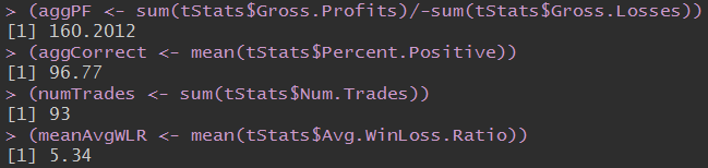
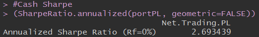
Though it made a relatively small amount of trades over 13 years, it boasts an impressive 2.7 Sharpe Ratio with 97% positive trades. Below on the left we can see the strategy’s performance vs. SPY (using very minimal leverage) and on the right the positions/trades are shown.

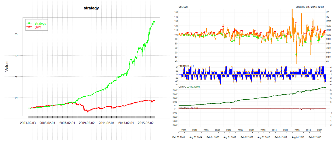
Overall, this definitely supports the potential of trading cointegrated ETF pairs with Bollinger Bands. I think it would be interesting to explore a form of position sizing based on either market volatility or the correlation between the ETF pair and another symbol/ETF. This concludes my analysis of cointegrated ETF pairs for now.

Acknowledgments: Thank you to Brian Peterson and Ernest Chan for explaining how to calculate the minimum capital required to trade a spread. Additionally, all of my blog posts have been edited prior to being published by Karin Muggli, so a huge thank you to her!

Note: I’m currently looking for a full-time quantitative research/trading position beginning summer/fall 2017. I’m currently a senior at the University of Washington, majoring in Industrial and Systems Engineering and minoring in Applied Mathematics. I also have taken upper level computer science classes and am proficient in a variety of programming languages. Resume: https://www.pdf-archive.com/2017/01/31/coltonsmith-resume-g/. LinkedIn: https://www.linkedin.com/in/coltonfsmith. Please let me know of any open positions that would be a good fit for me. Thanks!

Full Code:

detach("package:dplyr", unload=TRUE)
require(quantstrat)
require(IKTrading)
require(DSTrading)
require(knitr)
require(PerformanceAnalytics)
require(quantstrat)
require(tseries)
require(roll)
require(ggplot2)

# Full test
initDate="1990-01-01"
from="2003-01-01"
to="2015-12-31"

## Create "symbols" for Quanstrat
## adj1 = EWA (Australia), adj2 = EWC (Canada)

## Get data
getSymbols("EWA", from=from, to=to)
getSymbols("EWC", from=from, to=to)
dates = index(EWA)

adj1 = unclass(EWA$EWA.Adjusted)
adj2 = unclass(EWC$EWC.Adjusted)

## Ratio (EWC/EWA)
ratio = adj2/adj1

## Rolling regression
window = 21
lm = roll_lm(adj2,adj1,window)

## Plot beta
rollingbeta <- fortify.zoo(lm$coefficients[,2],melt=TRUE)
ggplot(rollingbeta, ylab="beta", xlab="time") + geom_line(aes(x=Index,y=Value)) + theme_bw()

## Calculate the spread
sprd <- vector(length=3273-21)
for (i in 21:3273) {
sprd[i-21] = (adj1[i]-rollingbeta[i,3]*adj2[i]) + 98.86608 ## Make the mean 100
}
plot(sprd, type="l", xlab="2003 to 2016", ylab="EWA-hedge*EWC")

## Find minimum capital
hedgeRatio = ratio*rollingbeta$Value*100
spreadPrice = 0.5*abs(adj2*100+adj1*hedgeRatio)
plot(spreadPrice, type="l", xlab="2003 to 2016", ylab="0.5*(abs(EWA*100+EWC*calculatedShares))")

## Combine columns and turn into xts
close = sprd
date = as.data.frame(dates[22:3273])
data = cbind(date, close)
dfdata = as.data.frame(data)
xtsData = xts(dfdata, order.by=as.Date(dfdata$date))
xtsData$close = as.numeric(xtsData$close)
xtsData$dum = vector(length = 3252)
xtsData$dum = NULL
xtsData$dates.22.3273. = NULL

## Add SMA, moving stdev, and z-score
rollz<-function(x,n){
avg=rollapply(x, n, mean)
std=rollapply(x, n, sd)
z=(x-avg)/std
return(z)
}

## Varying the lookback has a large affect on the data
xtsData$zScore = rollz(xtsData,50)
symbols = 'xtsData'

## Backtest
currency('USD')
Sys.setenv(TZ="UTC")
stock(symbols, currency="USD", multiplier=1)

#trade sizing and initial equity settings
tradeSize <- 10000
initEq <- tradeSize

strategy.st <- portfolio.st <- account.st <- "EWA_EWC"
rm.strat(portfolio.st)
rm.strat(strategy.st)
initPortf(portfolio.st, symbols=symbols, initDate=initDate, currency='USD')
initAcct(account.st, portfolios=portfolio.st, initDate=initDate, currency='USD',initEq=initEq)
initOrders(portfolio.st, initDate=initDate)
strategy(strategy.st, store=TRUE)

#SIGNALS
add.signal(strategy = strategy.st,
name="sigFormula",
arguments = list(label = "enterLong",
formula = "zScore < -1", cross = TRUE), label = "enterLong") add.signal(strategy = strategy.st, name="sigFormula", arguments = list(label = "exitLong", formula = "zScore > 1",
cross = TRUE),
label = "exitLong")

add.signal(strategy = strategy.st,
name="sigFormula",
arguments = list(label = "enterShort",
formula = "zScore > 1",
cross = TRUE),
label = "enterShort")

add.signal(strategy = strategy.st,
name="sigFormula",
arguments = list(label = "exitShort",
formula = "zScore < -1",
cross = TRUE),
label = "exitShort")

#RULES
add.rule(strategy = strategy.st,
name = "ruleSignal",
arguments = list(sigcol = "enterLong",
sigval = TRUE,
orderqty = 15,
ordertype = "market",
orderside = "long",
replace = FALSE,
threshold = NULL),
type = "enter")

add.rule(strategy = strategy.st,
name = "ruleSignal",
arguments = list(sigcol = "exitLong",
sigval = TRUE,
orderqty = "all",
ordertype = "market",
orderside = "long",
replace = FALSE,
threshold = NULL),
type = "exit")

add.rule(strategy = strategy.st,
name = "ruleSignal",
arguments = list(sigcol = "enterShort",
sigval = TRUE,
orderqty = -15,
ordertype = "market",
orderside = "short",
replace = FALSE,
threshold = NULL),
type = "enter")

add.rule(strategy = strategy.st,
name = "ruleSignal",
arguments = list(sigcol = "exitShort",
sigval = TRUE,
orderqty = "all",
ordertype = "market",
orderside = "short",
replace = FALSE,
threshold = NULL),
type = "exit")

#apply strategy
t1 <- Sys.time()
out <- applyStrategy(strategy=strategy.st,portfolios=portfolio.st)
t2 <- Sys.time()
print(t2-t1)

#set up analytics
updatePortf(portfolio.st)
dateRange <- time(getPortfolio(portfolio.st)$summary)[-1]
updateAcct(portfolio.st,dateRange)
updateEndEq(account.st)

#Stats
tStats <- tradeStats(Portfolios = portfolio.st, use="trades", inclZeroDays=FALSE)
tStats[,4:ncol(tStats)] <- round(tStats[,4:ncol(tStats)], 2)
print(data.frame(t(tStats[,-c(1,2)])))

#Averages
(aggPF <- sum(tStats$Gross.Profits)/-sum(tStats$Gross.Losses))
(aggCorrect <- mean(tStats$Percent.Positive))
(numTrades <- sum(tStats$Num.Trades))
(meanAvgWLR <- mean(tStats$Avg.WinLoss.Ratio))

#portfolio cash PL
portPL <- .blotter$portfolio.EWA_EWC$summary$Net.Trading.PL

## Sharpe Ratio
(SharpeRatio.annualized(portPL, geometric=FALSE))

## Performance vs. SPY
instRets <- PortfReturns(account.st)
portfRets <- xts(rowMeans(instRets)*ncol(instRets), order.by=index(instRets))

cumPortfRets <- cumprod(1+portfRets)
firstNonZeroDay <- index(portfRets)[min(which(portfRets!=0))]
getSymbols("SPY", from=firstNonZeroDay, to="2015-12-31")
SPYrets <- diff(log(Cl(SPY)))[-1]
cumSPYrets <- cumprod(1+SPYrets)
comparison <- cbind(cumPortfRets, cumSPYrets)
colnames(comparison) <- c("strategy", "SPY")
chart.TimeSeries(comparison, legend.loc = "topleft", colorset = c("green","red"))

## Chart Position
rets <- PortfReturns(Account = account.st)
rownames(rets) <- NULL
charts.PerformanceSummary(rets, colorset = bluefocus)

The next two blog posts will explore the basics of the statistical arbitrage strategies outlined in Ernest Chan’s book, Algorithmic Trading: Winning Strategies and Their Rationale. In the first post we will construct mean reverting time series data from cointegrated ETF pairs. The two pairs we will analyze are EWA (Australia) – EWC (Canada) and IGE (NA Natural Resources) – EWZ (Brazil).

EWA-EWC is a notable ETF pair since both Australia and Canada’s economies are commodity based. Looking at the scatter plot, it seems likely that they cointegrate because of this. IGE-EWZ seems less likely to cointegrate but we will discover that it is possible to salvage a stationary series with a statistical adjustment. A stationary, mean reverting series implies that the variance of the log price increases slower than that of a geometric random walk.

Running a linear regression model with EWA as the dependent variable and EWC as the independent variable we can use the resulting beta as the hedge ratio to create the data series below.

It appears stationary but we will run a few statistical tests to support this conclusion. The first test we will run is the Augmented Dickey-Fuller, which tests whether the data is stationary or trending. We set the lag parameter, k, to 1 since the change in price often has serial correlations.

The ADF test rejects the null hypothesis and supports the stationarity of the series with a p-value < 0.04. The next test we will run is the Hurst Exponent, which will analyze the variance of the log price and compare it to that of a geometric random walk. A geometric random walk has H=0.5, a mean reverting series has H<0.5, and a trending series has H>0.5. Running this test on the log residuals of the linear model gives a Hurst Exponent of 0.27, supporting the ADF’s conclusion. Since this series is now surely stationary, the final analysis we will do is find its half-life of the mean reversion. This is useful for trading as it gives you an idea of what the holding period of the strategy will be. The calculation of the half-life involves regressing y(t)-y(t-1) against y(t-1) and using the lambda found. See my code for further explanation. The half-life of this series is found to be 67 days.

Next, we will look at the IGE-EWZ pair. Running a linear regression model with IGE as the dependent variable and EWZ as the independent variable we can use the resulting beta as the hedge ratio to create the data series below.

Compared to the EWA-EWC pair, this looks a lot less stationary which makes sense considering the price series and scatter plot. Additionally, the ADF test is inconclusive.

The half-life of its mean reversion is calculated to be 344 days. In this form, it is definitely not a very practical pair to trade. Something that may improve the stationarity of this time series is to use an adaptive hedge ratio, determined from using a rolling linear regression model with a designated lookback window. Obviously, the shorter the lookback window, the more that the beta/hedge ratio will fluctuate. Though this would require daily portfolio adjustments, ideally the stationarity of the series will increase substantially. I began with a lookback window of 252, the number of trading days in a year, but it didn’t have large enough of an impact.  Therefore, we will try 21, the average number of trading days in a month, which will result in a significant impact. Without the rolling regression, the beta/hedge ratio was 0.42. Below you can see how the beta changes over time and how it affects the mean reverting data series.

With the adaptive hedge ratio, the ADF test strongly concludes that the time series is stationary. This also significantly cuts down the half-life of the mean reversion to only 33 days.

Though there are a lot more analysis techniques for cointegrated ETF pairs, and even triplets, this post explored the basics of creating two stationary data series. In next week’s post, we will implement some mean reversion trading strategies on these pairs. See ya next week!

Full Code:

require(quantstrat)
require(tseries)
require(roll)
require(ggplot2)

## EWA (Australia) - EWC (Canada)
## Get data
getSymbols("EWA", from="2003-01-01", to="2015-12-31")
getSymbols("EWC", from="2003-01-01", to="2015-12-31")

## Utilize the backwards-adjusted closing prices
adj1 = unclass(EWA$EWA.Adjusted)
adj2 = unclass(EWC$EWC.Adjusted)

## Plot the ETF backward-adjusted closing prices
plot(adj1, type="l", xlab="2003 to 2016", ylab="ETF Backward-Adjusted Price in USD", col="blue")
par(new=T)
plot(adj2, type="l", axes=F, xlab="", ylab="", col="red")
par(new=F)

## Plot a scatter graph of the ETF adjusted prices
plot(adj1, adj2, xlab="EWA Backward-Adjusted Prices", ylab="EWC Backward-Adjusted Prices")

## Linear regression, dependent ~ independent
comb1 = lm(adj1~adj2)

## Plot the residuals or hedged pair
plot(comb1$residuals, type="l", xlab="2003 to 2016", ylab="Residuals of EWA and EWC regression")

beta = coef(comb1)[2]
X = vector(length = 3273)
for (i in 1:3273) {
X[i]=adj1[i]-beta*adj2[i]
}

plot(X, type="l", xlab="2003 to 2016", ylab="EWA-hedge*EWC")

## ADF test on the residuals
adf.test(comb1$residuals, k=1)
adf.test(X, k=1)

## Hurst Exponent Test
HurstIndex(log(comb1$residuals))

## Half-life
sprd = comb1$residuals
prev_sprd <- c(sprd[2:length(sprd)], 0)
d_sprd <- sprd - prev_sprd
prev_sprd_mean <- prev_sprd - mean(prev_sprd)
sprd.zoo <- merge(d_sprd, prev_sprd_mean)
sprd_t <- as.data.frame(sprd.zoo)

result <- lm(d_sprd ~ prev_sprd_mean, data = sprd_t)
half_life <- -log(2)/coef(result)[2]

#######################################################################################################

## EWZ (Brazil) - IGE (NA Natural Resource)
## Get data
getSymbols("EWZ", from="2003-01-01", to="2015-12-31")
getSymbols("IGE", from="2003-01-01", to="2015-12-31")

## Utilize the backwards-adjusted closing prices
adj1 = unclass(EWZ$EWZ.Adjusted)
adj2 = unclass(IGE$IGE.Adjusted)

## Plot the ETF backward-adjusted closing prices
plot(adj1, type="l", xlab="2003 to 2016", ylab="ETF Backward-Adjusted Price in USD", col="blue")
par(new=T)
plot(adj2, type="l", axes=F, xlab="", ylab="", col="red")
par(new=F)

## Plot a scatter graph of the ETF adjusted prices
plot(adj1, adj2, xlab="EWA Backward-Adjusted Prices", ylab="EWC Backward-Adjusted Prices")

## Rolling regression
## Trading days
## 252 = year
## 21 = month
window = 21
lm = roll_lm(adj1,adj2,window)

## Plot beta
rollingbeta <- fortify.zoo(lm$coefficients[,2],melt=TRUE)
ggplot(rollingbeta, ylab="beta", xlab="time") + geom_line(aes(x=Index,y=Value)) + theme_bw()

## X should be the shifted residuals
X <- vector(length=3273-21)
for (i in 21:3273) {
X[i-21] = adj2[i]-rollingbeta[i,3]*adj1[i]
}

plot(X, type="l", xlab="2003 to 2016", ylab="IGE-hedge*EWZ")