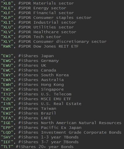
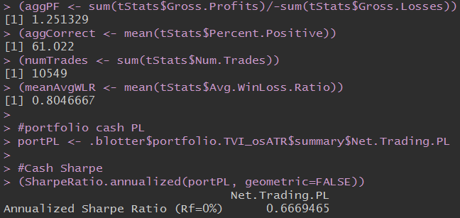
Finally a somewhat profitable strategy to analyze! This post will walk through the development of my MACD + SMI strategy, including my experience with parameter optimization and trailing stops. This strategy began with an interest in the Moving Average Convergence/Divergence oscillator (MACD), which I hadn’t yet explored. Also, since the two previous strategies I analyzed were mean-reversion strategies, I thought it’d be good to try out a trend-following strategy. The MACD uses two trend-following moving averages to create a momentum indicator. I used the standard 12-period fast EMA, 26-period slow EMA, and 9-period signal EMA parameters. Although there are a lot of different signals that traders can look at when using the MACD, I kept it simple and was only interested when the MACD (fast EMA – slow EMA) was above/below the signal line. When the MACD is positive it indicates that the upside momentum is increasing, and vice versa for negative values. I then did some research to see what indicators were combined with the MACD. The two that caught my interest were the Stochastic Momentum Index (SMI) and the Chande Momentum Oscillator (CMO). The SMI compares closing prices to the median of the high/low range of prices over a certain period, which makes it a more refined and sensitive version of the Stochastic Oscillator. The values range between -100 and +100, with values less than -40 indicating a bearish trend and values greater than 40 indicating a bullish trend. Normally the SMI can be used similarly to the RSI and indicate overbought/oversold market conditions, but I wanted to focus on using it as a general trend indicator. The CMO indicator is also a momentum oscillator that can be used to confirm possible trends; my backtests confirmed its viability but I decided to center my focus on the SMI. I initially used the standard SMI threshold values (-40/+40) and backtested across the same 30 ETFs from my last post during 2003-2015.
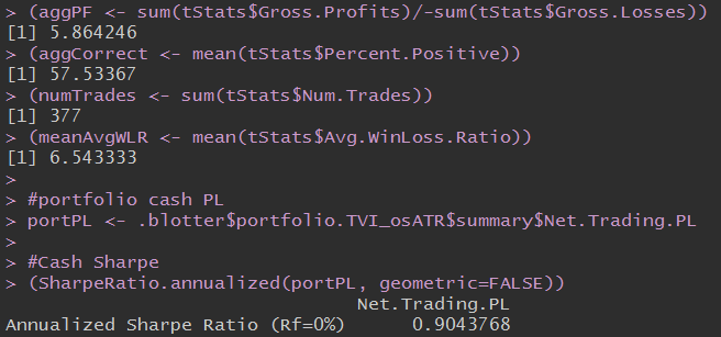
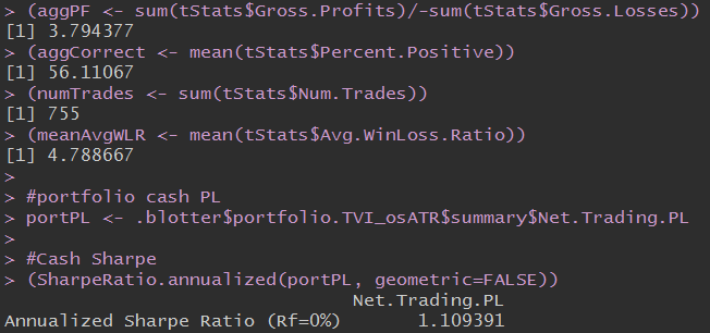
This was my first time seeing such a high profit factor and a Sharpe ratio fairly close to 1, but unfortunately, the number of trades was too low. A minimum of 700/800 trades is necessary in this backtest to support strategy performance conclusions, however I was happy to see signs of a profitable strategy. As a note, ATR position sizing was used in every strategy backtest, which nearly doubles their Sharpe Ratio. To increase the number of trades made by this strategy I had a couple of ideas. First, since this strategy only enters long positions I tried playing around with the indicators to see if it was also good for entering short positions. This unfortunately was not a profitable attempt. Second, I thought about exploring a separate shorting strategy that made ~400 trades, and simply putting them together. I decided for the sake of analysis it would be better to stick to one main strategy this time, but this is something I’ll consider in the future. Third and finally, after learning about the ATR position sizing I have wanted to experiment with another risk management tool, trailing stops. I added a 7% trailing stop and got the results below. It sacrificed some profit factor for a better Sharpe ratio, but it also made over 700 trades. Although this seems like artificially increasing the number of trades, I was content with the results for the time being.
Next, I wanted to see if I could push that profit factor over 4 by optimizing the parameters, namely the SMI thresholds and trailing stop percentages. I did minor parameter optimization in my first post, but this was my first time doing it on a larger scale. I decided to split my time period in half, 2003-2009 and 2010-2015, optimize on the first period, and then use the second period for an out of sample test. I didn’t expect to see a large difference of performance between the two periods, but I was very wrong. I decided to first optimize the SMI thresholds and found ridiculously large profit factors. From this I concluded that 40 was the best entrance, but that the exit signal definitely had the largest impact. I then chose to further optimize the 40/55 (highest profit factor), 40/30 (highest Sharpe ratio), and 40/40 (arguably the best mix of profit factor and Sharpe ratio to support why they’re the standard thresholds).
| Optimization 2003-2009 | ||||
| SMI Enter (+) | SMI Close (-) | Profit Factor | Trades | Sharpe Ratio |
| 40 | 45 | 14.92 | 152 | 1.13 |
| 40 | 50 | 18.25 | 127 | 0.99 |
| 40 | 35 | 9.25 | 225 | 1.24 |
| 40 | 30 | 8.18 | 258 | 1.29 |
| 40 | 55 | 22.14 | 105 | 0.91 |
| 40 | 40 | 11.29 | 191 | 1.24 |
| 35 | 40 | 10.33 | 201 | 1.25 |
| 30 | 40 | 9.94 | 210 | 1.27 |
| 45 | 40 | 11.12 | 185 | 1.22 |
| 50 | 40 | 10.49 | 179 | 1.17 |
Then I tested the 3 strategies with 5%, 10%, 15%, and 20% trailing stops. Based on their performance, I decided which ones to test on the out of sample period and the whole sample period.
| Optimization 2003-2009 | ||||||
| SMI Enter (+) | SMI Close (-) | Trailing Stop | Profit Factor | Trades | Sharpe Ratio | Continue? |
| 40 | 40 | 5% | 4.95 | 535 | 1.67 | * |
| 40 | 40 | 10% | 7.49 | 307 | 1.51 | * |
| 40 | 40 | 15% | 7.94 | 248 | 1.36 | |
| 40 | 40 | 20% | 9.22 | 213 | 1.33 | * |
| 40 | 55 | 5% | 5.06 | 528 | 1.7 | * |
| 40 | 55 | 10% | 8.4 | 286 | 1.53 | * |
| 40 | 55 | 15% | 9.45 | 207 | 1.4 | |
| 40 | 55 | 20% | 10.85 | 163 | 1.3 | * |
| 40 | 30 | 5% | 4.97 | 539 | 1.7 | * |
| 40 | 30 | 10% | 6.82 | 335 | 1.51 | |
| 40 | 30 | 15% | – | – | – | |
| 40 | 30 | 20% | – | – | – | |
| OOS 2010-2015 | ||||||
| SMI Enter (+) | SMI Close (-) | Trailing Stop | Profit Factor | Trades | Sharpe Ratio | Continue? |
| 40 | 40 | 5% | 2.3 | 436 | 0.77 | * |
| 40 | 40 | 10% | 2.23 | 277 | 0.53 | * |
| 40 | 40 | 15% | – | – | – | |
| 40 | 40 | 20% | 2.23 | 221 | 0.48 | |
| 40 | 55 | 0.05 | 2.45 | 430 | 0.82 | * |
| 40 | 55 | 10% | 2.84 | 244 | 0.68 | * |
| 40 | 55 | 15% | – | – | – | |
| 40 | 55 | 20% | 3.92 | 146 | 0.63 | |
| 40 | 30 | 5% | 2.17 | 447 | 0.71 | * |
| 40 | 30 | 10% | – | – | – | |
| 40 | 30 | 15% | – | – | – | |
| 40 | 30 | 20% | – | – | – | |
| Whole Period | |||||
| SMI Enter (+) | SMI Close (-) | Trailing Stop | Profit Factor | Trades | Sharpe Ratio |
| 40 | 40 | 5% | 3.38 | 977 | 1.23 |
| 40 | 40 | 10% | 3.95 | 586 | 1.01 |
| 40 | 40 | 15% | – | – | – |
| 40 | 40 | 20% | – | – | – |
| 40 | 55 | 0.05 | 3.54 | 963 | 1.27 |
| 40 | 55 | 10% | 4.65 | 531 | 1.09 |
| 40 | 55 | 15% | – | – | – |
| 40 | 55 | 20% | – | – | – |
| 40 | 30 | 5% | 3.28 | 993 | 1.21 |
| 40 | 30 | 10% | – | – | – |
| 40 | 30 | 15% | – | – | – |
| 40 | 30 | 20% | – | – | – |
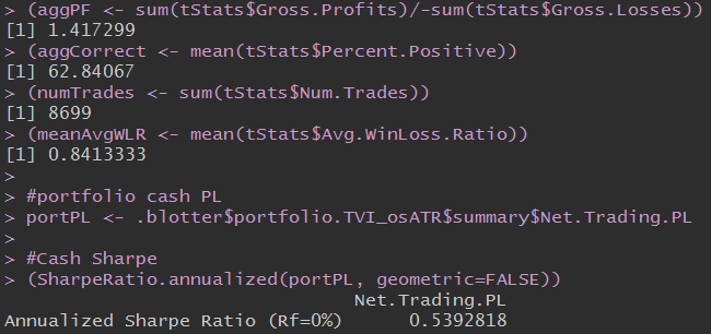
I was shocked at how much worse the strategies performed in the out of sample period compared to the optimization period. It was really quite interesting, and I suspect there had to be significantly different market conditions to make these differences apparent for all of the strategies. Across the board the best performing strategy was 40/55, with fairly impressive profit factors and Sharp ratios. The higher closing threshold is probably a result of the general upward trending market. This strategy performed best with a 5% or 10% trailing stop but it made almost double the trades with 5% so I decided to try my original 7% trailing stop. The results are below.
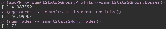
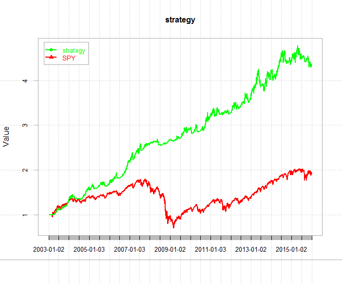
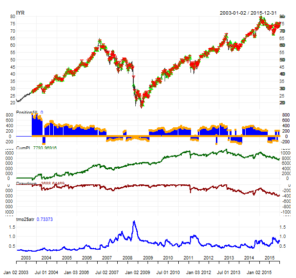
Overall, not a bad strategy, with a profit factor above 4 and a decent Sharpe Ratio. It also handled 2008 very nicely. The buy and hold inter-instrument correlation of the 30 ETFs is 0.71 and this strategy cuts it in half. This means it is a well diversified and risk managed portfolio strategy.

I’m going to continue to search for profitable strategies and maybe look for a short-term, aggressive strategy to analyze next. I also want to use other metrics, such as the Calmar or Information ratio instead of the Sharpe ratio to get a bigger picture of a strategy’s risk management. Additionally, I hope to apply R’s extensive machine learning capabilities to a strategy in the near future. Thanks for reading!
Acknowledgements: Thank you to Ilya Kipnis and Ernest Chan for their continual help.
Full code:
detach("package:dplyr", unload=TRUE)
require(quantstrat)
require(IKTrading)
require(DSTrading)
require(knitr)
require(PerformanceAnalytics)
# Full test
initDate="1990-01-01"
from="2003-01-01"
to="2015-12-31"
# Optimization set
# initDate="1990-01-01"
# from="2003-01-01"
# to="2009-12-31"
# OOS test
# initDate="1990-01-01"
# from="2010-01-01"
# to="2015-12-31"
#to rerun the strategy, rerun everything below this line
source("demoData.R") #contains all of the data-related boilerplate.
#trade sizing and initial equity settings
tradeSize <- 10000
initEq <- tradeSize*length(symbols)
strategy.st <- portfolio.st <- account.st <- "TVI_osATR"
rm.strat(portfolio.st)
rm.strat(strategy.st)
initPortf(portfolio.st, symbols=symbols, initDate=initDate, currency='USD')
initAcct(account.st, portfolios=portfolio.st, initDate=initDate, currency='USD',initEq=initEq)
initOrders(portfolio.st, initDate=initDate)
strategy(strategy.st, store=TRUE)
#parameters (trigger lag unchanged, defaulted at 1)
period = 20
pctATR = .02 #control risk with this parameter
trailingStopPercent = 0.07
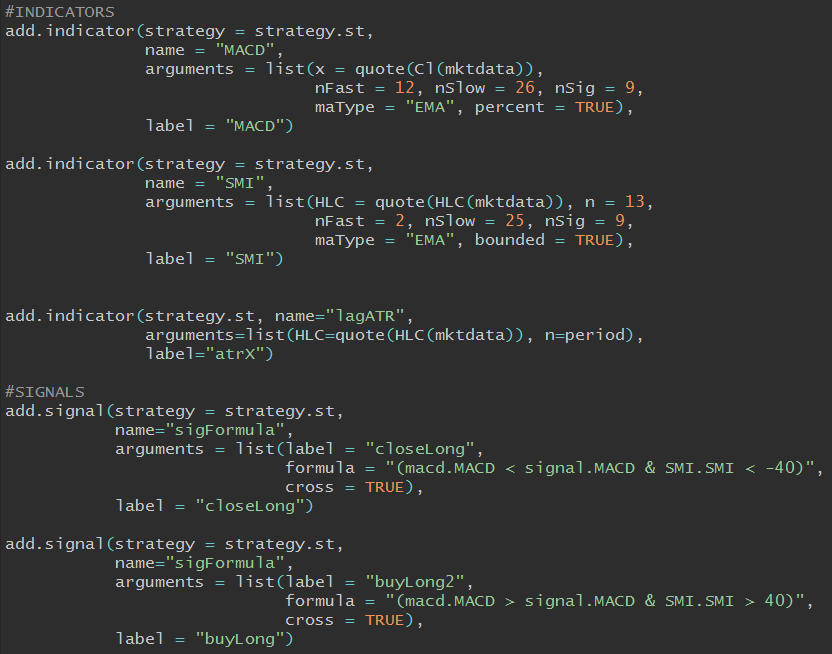
#INDICATORS
add.indicator(strategy = strategy.st,
name = "MACD",
arguments = list(x = quote(Cl(mktdata)),
nFast = 12, nSlow = 26, nSig = 9,
maType = "EMA", percent = TRUE),
label = "MACD")
add.indicator(strategy = strategy.st,
name = "SMI",
arguments = list(HLC = quote(HLC(mktdata)), n = 13,
nFast = 2, nSlow = 25, nSig = 9,
maType = "EMA", bounded = TRUE),
label = "SMI")
add.indicator(strategy.st, name="lagATR",
arguments=list(HLC=quote(HLC(mktdata)), n=period),
label="atrX")
#SIGNALS
add.signal(strategy = strategy.st,
name="sigFormula",
arguments = list(label = "closeLong",
formula = "(macd.MACD < signal.MACD & SMI.SMI < -55)",
cross = TRUE),
label = "closeLong")
add.signal(strategy = strategy.st,
name="sigFormula",
arguments = list(label = "buyLong",
formula = "(macd.MACD > signal.MACD & SMI.SMI > 40)",
cross = TRUE),
label = "buyLong")
#RULES
add.rule(strategy = strategy.st,
name = "ruleSignal",
arguments = list(sigcol = "buyLong",
sigval = TRUE,
ordertype = "market",
orderside = "long",
replace=FALSE, prefer="Open", osFUN=osDollarATR,
tradeSize=tradeSize, pctATR=pctATR, atrMod="X"),
type="enter", path.dep=TRUE, label = "LE")
add.rule(strategy = strategy.st,
name = "ruleSignal",
arguments = list(sigcol = "buyLong",
sigval = TRUE,
replace = FALSE,
orderside = "long",
ordertype = "stoptrailing",
tmult = TRUE,
threshold = quote(trailingStopPercent),
orderqty = "all",
orderset = "ocolong"),
type = "chain",
parent = "LE",
label = "StopTrailingLong",
enabled = FALSE)
add.rule(strategy = strategy.st,
name = "ruleSignal",
arguments = list(sigcol = "closeLong",
sigval = TRUE,
orderqty = "all",
ordertype = "market",
orderside = "long",
threshold = NULL),
type = "exit")
enable.rule(strategy.st, type = "chain", label = "StopTrailingLong")
#apply strategy
t1 <- Sys.time()
out <- applyStrategy(strategy=strategy.st,portfolios=portfolio.st)
t2 <- Sys.time()
print(t2-t1)
#set up analytics
updatePortf(portfolio.st)
dateRange <- time(getPortfolio(portfolio.st)$summary)[-1]
updateAcct(portfolio.st,dateRange)
updateEndEq(account.st)
#Stats
tStats <- tradeStats(Portfolios = portfolio.st, use="trades", inclZeroDays=FALSE)
tStats[,4:ncol(tStats)] <- round(tStats[,4:ncol(tStats)], 2)
print(data.frame(t(tStats[,-c(1,2)])))
#Averages
(aggPF <- sum(tStats$Gross.Profits)/-sum(tStats$Gross.Losses))
(aggCorrect <- mean(tStats$Percent.Positive))
(numTrades <- sum(tStats$Num.Trades))
(meanAvgWLR <- mean(tStats$Avg.WinLoss.Ratio))
#portfolio cash PL
portPL <- .blotter$portfolio.TVI_osATR$summary$Net.Trading.PL
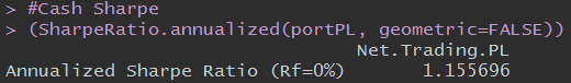
#Cash Sharpe
(SharpeRatio.annualized(portPL, geometric=FALSE))
#Individual instrument equity curve
# chart.Posn(portfolio.st, "IYR")
instRets <- PortfReturns(account.st)
portfRets <- xts(rowMeans(instRets)*ncol(instRets), order.by=index(instRets))
cumPortfRets <- cumprod(1+portfRets)
firstNonZeroDay <- index(portfRets)[min(which(portfRets!=0))]
getSymbols("SPY", from=firstNonZeroDay, to="2015-12-31")
SPYrets <- diff(log(Cl(SPY)))[-1]
cumSPYrets <- cumprod(1+SPYrets)
comparison <- cbind(cumPortfRets, cumSPYrets)
colnames(comparison) <- c("strategy", "SPY")
chart.TimeSeries(comparison, legend.loc = "topleft", colorset = c("green","red"))
#Correlations
instCors <- cor(instRets)
diag(instRets) <- NA
corMeans <- rowMeans(instCors, na.rm=TRUE)
names(corMeans) <- gsub(".DailyEndEq", "", names(corMeans))
print(round(corMeans,3))
mean(corMeans)