Category: Quantitative Finance

Using the Dynamic Mode Decomposition (DMD) to Rotate Long-Short Exposure Between Stock Market Sectors

Part 1 – Theoretical Background

The Dynamic Mode Decomposition (DMD) was originally developed for its application in fluid dynamics where it could decompose complex flows into simpler low-rank spatio-temporal features. The power of this method lies in the fact that it does not depend on any principle equations of the dynamic system it is analyzing and is thus equation-free [1]. Also, unlike other low-rank reconstruction algorithms like the Singular Value Decomposition (SVD), the DMD can be used to make short-term future state predictions.

The algorithm is implemented as follows [2].

1. We begin with a ${N}$ x ${M}$ matrix, ${\mathbf{X}}$ , containing data collected from ${N}$ sources over ${M}$ evenly spaced time periods, from the system of interest.

2. From this matrix two sub-matrices are constructed, ${\mathbf{X}_1^{M-1}}$ and ${\mathbf{X}_2^M}$ , which are defined below.

$\displaystyle \mathbf{X}_j^k = \begin{bmatrix} \mathbf{x}(t_j) & \mathbf{x}(t_{j+1}) & ... & \mathbf{x}(t_k) \end{bmatrix}$
$\displaystyle \mathbf{X}_1^{M-1} = \begin{bmatrix} \mathbf{x}_1 & \mathbf{x}_2 & ... & \mathbf{x}_{M-1} \end{bmatrix}$
$\displaystyle \mathbf{X}_2^{M} = \begin{bmatrix} \mathbf{x}_2 & \mathbf{x}_3 & ... & \mathbf{x}_{M} \end{bmatrix}$

We can consider a Koopman operator ${\mathbf{A}}$ such that ${\mathbf{x}_{j+1} = \mathbf{Ax}_j}$ and rewrite ${\mathbf{X}_1^{M-1}}$ as

$\displaystyle \mathbf{X}_1^{M-1} = \begin{bmatrix} \mathbf{x}_1 & \mathbf{A}\mathbf{x}_1 & ... & \mathbf{A}^{M-2}\mathbf{x}_1 \end{bmatrix}$

whose columns now are elements in a Krylov space.

3. The SVD decomposition of ${\mathbf{X}_1^{M-1}}$ is computed.

$\displaystyle \mathbf{X}_1^{M-1} = \mathbf{U \Sigma V^*}$

Then based on the variance captured by the singular values and the application of the algorithm, the number of desired reconstructions ranks can be chosen.

4. The matrix ${\mathbf{A}}$ is constructed such that it is the best mapping between the two sub-matrices.

$\displaystyle \mathbf{A}\mathbf{X}_1^{M-1} \approx \mathbf{X}_2^M$

${\mathbf{A}}$ can be approximated with ${\mathbf{\tilde{A}}}$ from evaluating the expression

$\displaystyle \mathbf{\tilde{A}} = \mathbf{U^*X_2^M V\Sigma^{-1}}$

where ${\mathbf{U}}$ , ${\mathbf{\Sigma}}$ , and ${\mathbf{V}}$ are the truncated matrices from the SVD reduction of ${\mathbf{X}_1^{M-1}}$ . The eigenvalue problem associated with ${\mathbf{\tilde{A}}}$ is

$\displaystyle \mathbf{\tilde{A}}\mathbf{y}_k = \mu_k \mathbf{y}_k \qquad k = 1,2,..,K$

where ${K}$ is the rank of approximation that was chosen previously. The eigenvalues ${\mu_k}$ contain information on the time dynamics of our system and the eigenvectors can be used to construct the DMD modes.

$\displaystyle \mathbf{\psi}_k = \mathbf{Uy}_k$

5. The approximated solution for all future times, ${\mathbf{x}_{DMD}(t)}$ , can now be written as

$\displaystyle \mathbf{x}_{DMD}(t) = \sum_{k=1}^K b_k(0) \mathbf{\psi}_k(\mathbf{x}) \exp{(\omega_k t)} = \mathbf{\Psi} \text{diag}(\exp{(\omega t)}) \mathbf{b}$

where ${\omega_k = \ln(\mu_k)/\Delta t}$ , ${b_k(0)}$ is the initial amplitude of each mode, ${\mathbf{\Psi}}$ is the matrix whose columns are eigenvectors ${\mathbf{\psi}_k}$ , and ${\mathbf{b}}$ is the vector of coefficients. Finally, all that needs to be computed is the initial coefficient values ${b_k(0)}$ which can be found by looking at time zero and solving for ${\mathbf{b}}$ via a pseudo-inverse in the equation

$\displaystyle \mathbf{x_0} = \mathbf{\Psi b}$

To summarize the algorithm, we will “train” a matrix ${\mathbf{\tilde{A}}}$ on a subset of the data whose eigenvalues and eigenvectors contain necessary information to make future state predictions for a given time horizon.

Part 2 – Basic Demonstration

We begin with a basic example to demonstrate how to use the pyDMD package. First, we construct a matrix $\mathbf{X}$ where each row is a snapshot in time and each column can be thought of as a different location in our system being sampled.

$\displaystyle \mathbf{X} = \begin{bmatrix} -2 & 6 & 1 & 1 & -1 \\ -1 & 5 & 1 & 2 & -1 \\ 0 & 4 & 2 & 1 & -1 \\ 1 & 3 & 2 & 2 & -1 \\ 2 & 2 & 3 & 1 & -1 \\ 3 & 1 & 3 & 2 & -1 \\ \end{bmatrix}$

Now we will attempt to predict the predict the 6th row using a future state prediction from the DMD fitted on the first 5 rows.

import numpy as np
from pydmd import DMD
df = np.array([[-2,6,1,1,-1],
               [-1,5,1,2,-1],
               [0,4,2,1,-1],
               [1,3,2,2,-1],
               [2,2,3,1,-1],
               [3,1,3,2,-1]])

dmd = DMD(svd_rank = 2) # Specify desired truncation
train = df[:5,:]
dmd.fit(train.T) # Fit the model on the first 5 rows
dmd.dmd_time['tend'] *= (1+1/6) # Predict one additional time step
recon = dmd.reconstructed_data.real.T # Make prediction

print('Actual :',df[5,:])
print('Predicted :',recon[5,:])

Two SVD ranks were used for the reconstruction and the result is pleasantly accurate for how easily it was implemented.

$\displaystyle \mathbf{x_{True}}(6) = \begin{bmatrix} 3 & 1 & 3 & 2 & -1 \end{bmatrix}$

$\displaystyle \mathbf{x_{DMD}}(6) = \begin{bmatrix} 2.8 & 0.8 & 2.6 & 2.0 & -0.9 \end{bmatrix}$

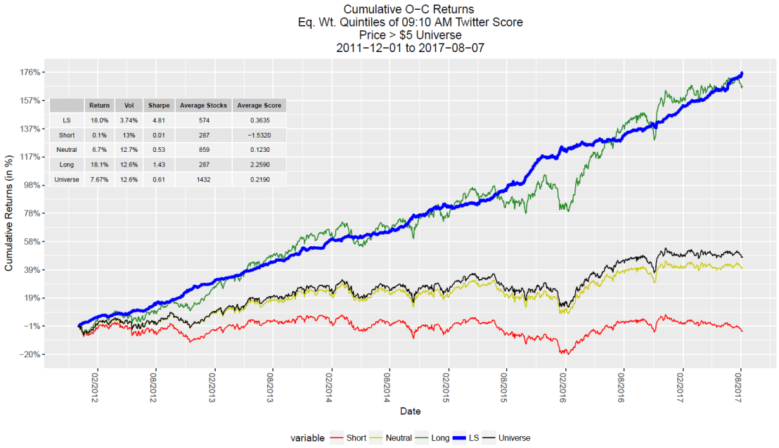
Part 3 – Sector Rotation Strategy

We will now attempt to model the stock market as a dynamic system broken down by sectors and use the DMD to predict which sectors to be long and short in over time. This is commonly known as a sector rotation strategy. To ensure that we have adequate historical data we will use 9 sector ETFs: XLY, XLP, XLE, XLF, XLV, XLI, XLB, XLK, and XLU from 2000-2019 and rebalance monthly. The strategy is implemented as follows:

Fit a DMD model using the last N months of monthly returns. The SVD rank reconstruction number can be chosen as desired.
Use the DMD model to predict the next month’s snapshot which are the returns of each ETF.
Construct the portfolio by taking long positions in the top 5 ETFs and short positions in the bottom 4 ETFs. Thus, we are remaining very close to market neutral.
Continue this over time by refitting the model monthly and making a new prediction for the next month.

Though the results are quite sensitive to changes in the model parameters, some of the best parameters achieve Sharpe ratios superior to the long only portfolio while remaining roughly market neutral which is very encouraging and warrants further exploration with a proper, robust backtest procedure.

Figure_1-1

The code and functions used to produce this plot can found here. There are also many additional features of the pyDMD package that we did not explore that could potentially improve the results. If you have any questions, feel free to reach out by email at coltonsmith321@gmail.com

References

[1] N. Kutz, S. Brunton, B. Brunton, and J. Proctor, Dynamic Mode Decomposition: Data-Driven Modeling of Complex Systems. 2016.

[2] Mann, Jordan & Nathan Kutz, J. Dynamic Mode Decomposition for Financial Trading Strategies. Quantitative Finance. 16. 10.1080/14697688.2016.1170194. 2015.

Constructing Continuous Futures Price Series

Welcome! If you enjoy these posts, please follow this blog via email and check out my Twitter feed located on the sidebar.

All of my previous analysis has focused on US equities, but today we begin the journey into another asset class, futures. Futures are traded via contracts where two parties agree to exchange a quantity of an asset for a price decided today and delivered at a specified date in the future. The expiration dates of the contracts vary based on the underlying asset and range from monthly to quarterly. To properly evaluate the profitability of trading strategies with historical futures contract data, it is necessary to combine these contracts into a continuous price series. This isn’t entirely straightforward because contango and backwardation factors cause contracts of the same underlying asset with different expiration dates to be priced differently. It is initially unclear how to best concatenate these price series, so I want to explore a few of the basic methods and their advantages. I’m interested in exploring futures strategies, so this was a necessary first step since Quandl’s free continuous futures data is of insufficient quality, but they provide high quality individual contract data. Becoming comfortable with the contract data while creating flexible, testable continuous price series is a valuable exercise. Additionally, I decided to use Python because I have not done a project with it and this is a useful applied problem to build some Python skills.

For this example, we will construct a variety of continuous price series for the commodity wheat. The first step is to pull the contract data from the Quandl API and store it appropriately (see the included code). To begin, let’s plot all the contracts’ prices to observe the behavior of the price data. As seen in Figure 1 below, although there is some consistency between the contracts, there is a significant amount of variance.

10.1 — Figure 1: Futures Prices of All Wheat Contracts

Ideally, to make this a backtest-ready series, we need to be trading a single contract at each point in time (or possibly a combination of contracts). The further we are from a contract’s expiration; the more price speculation is embedded into the price. The front or nearest month contract refers to the contract which has the soonest expiration date and thus has the least amount of speculation. Generally, front month contracts have the most trading activity, as measured by open interest. When expiration approaches, traders will roll their positions over to the next contract or let them expire. A basic approach to construct a continuous series would be to always use the front month contract’s price and when the current front month contract expires, switch to the new front month contract. There is one caveat, the price of the contracts when you rollover may not be the same, and in general, won’t be the same. These gaps will create artificial, untradeable price movements in the continuous series. To create a smooth transition between contracts, we can adjust them in such a way so that there won’t be a gap. We’ll refer to the size of this gap as the adjustment factor. Forward adjusting would shift the next contract to eliminate the gap by subtracting the adjustment factor from the next contract’s price series. Backward adjusting would shift the previous contract to eliminate the gap by adding the adjustment factor to the previous contract’s price series. Figure 2 below shows an example of these adjustments for an actual rollover.

Figure 2: Backward/Forward Adjusting Example

Now, when this approach is extended over multiple contracts the adjustment factors will simply cumulate so that prices for every contract are appropriately adjusted. The quality of the data is the same whether you backward or forward adjust. The difference is what needs to be recalculated with each new contract and what the values represent. The backward adjusted series’ current values represent the actual market values thus the historical data needs to be recalculated when a new contract is added to the series. The forward adjusted series does not require recalculating historical data but since each new contract that is added to the series needs to be adjusted, the new prices will not represent the actual market values. Figure 3 below shows the fully adjusted wheat series. Notice that the difference between the forward and backward adjusted series remains constant. This difference is the total adjustment factor.

10.3 — Figure 3: Expiration Adjusted Wheat Series

A point that becomes apparent, here, is that we are adjusting the price series, not the returns. The daily returns of the forward and backward adjusted series differ. When creating continuous prices, you are forced to choose between either correct P&L or correct returns. To adjust for correct returns, one would need to work with the daily log returns series of the contracts and then construct a usable price series from those. Dr. Ernest Chan’s second book covers this concept thoroughly on pg. 12-16.

Another approach to construct a continuous series is the perpetual method, which smooths the transitions between contracts by taking a weighted average of the contracts’ prices during the transition period. This can be weighted on time left to expiration, open interest, or other properties of the contracts. For this example, we will begin the transition to the next contract once its open interest becomes greater than the current contract and weight the prices during the transition based on open interest. As seen in Figure 4 below, this happens prior to the expiration of the contracts.

10.4 — Figure 4: 2014 Wheat Contracts’ Open Interest

Like the previous example, one could also forward/backward adjust using the open interest crossover date which is more realistic because of better liquidity. This option is available in the attached code. In our case, after this crossover date, we transition to the next contract over the next 5 days (the number of days is adjustable) based on open interest. Figure 5 below shows the slightly smoother perpetual adjusted series.

10.5 — Figure 5: Perpetual Adjusted Wheat Series

This smoothed price series may be advantageous for statistical research since it reduces noise in longer term signals but it contains prices that are not directly tradable. To trade the price during the transition period, one would have to rebalance their percentage of the current and next contract each day, which would incur transaction costs.

There are a variety of other adjustment methods, but the examples shown here provide a strong and sufficient foundation. A paper that I found very helpful and one that covers additional methods is available here. The Python code accompanying this post can be found here. I hope you found these examples helpful. In my next post, I am going to use these continuous series as I analyze futures trading strategies. Thanks for reading!

Cointegration, Correlation, and Log Returns

Co-Author: Eric Kammers

I recently created a Twitter account for the blog where I will curate and comment on content I find interesting related to finance, data science, and data visualization. Please follow me at @Quantoisseur (see the embedded stream on the sidebar). Enjoy the post!

The differences between correlation and cointegration can often be confusing. While there are some helpful explanations online, I wasn’t satisfied with the visual examples. When looking at a plot of an actual pair of symbols where the correlation and cointegration test results differ, it can be difficult to pinpoint which portions of the time series are responsible for these separate properties. To solve this, I decided to produce some basic examples with sinusoidal functions so I could solidify my understanding of these concepts.

First, let’s highlight the difference between cointegration and correlation. Correlation is more familiar to most of us, especially outside of the financial industry. Correlation is a measure of how well two variables move in tandem together over time. Two common correlation measures are Pearson’s product-moment coefficient and Spearman’s ranks-order coefficient. Both coefficients range from -1, perfect negative correlation, to 0, no correlation, to 1, perfect positive correlation. Positive correlation means that the variables move in tandem in the same direction while negative correlation means that they move in tandem but in opposite directions. When calculating correlation, we look at returns rather than price because returns are normalized across differently priced assets. The main difference between the two correlation coefficients is that the Spearman coefficient measures the monotonic relationship between two variables, while the Pearson coefficient measures their linear relationship. Figure 1 below shows how the different coefficients behave when two variables exhibit either a linear or nonlinear relationship. Notice how the Spearman coefficient remains 1 for both scenarios since the relationship in both cases is perfectly monotonic.

fig1 — Figure 1: Pearson vs Spearman for Nonlinear and Linear Functions

Based on the distributions of the data, these coefficients can behave differently which I will explore with additional examples later in this post. Here are some resources for further clarification on the Pearson and Spearman coefficients.

Now, cointegration tests do not measure how well two variables move together, but rather whether the difference between their means remains constant. Often, variables with high correlation will also be cointegrated, and vice versa, but this isn’t always the case. In contrast to correlation, when testing for cointegration we use prices rather than returns since we’re more interested in the trend between the variables’ means over time than in the individual price movements. There are multiple cointegration tests, but in this case, I’ll be using the Augmented Dicky-Fuller test to evaluate the stationarity of the residuals from the linear model created with the pair’s price series.

Second, using log returns for financial calculations is, in many cases, preferable to using simple returns. There are many resources online explaining the advantages and disadvantages of using log returns. We will not dive into this topic too much, but some of the advantages are due to assuming a log normal distribution which makes them easier to work with and gives them convenient properties like time-additivity. Figure 2 below shows the relationship between log and simple returns.

fig2 — Figure 2: Relationship between Simple and Log Returns

Furthermore, correlation is a second moment calculation meaning that it is only appropriate if higher moments are insignificant. Using log returns is better so we can ensure the higher moments are negligible and avoid having to use copulas.

Now with this framework, we can introduce some visual examples. Figure 3 below will be our baseline example which we will adjust in a variety of ways to examine how the values in the table react. In this figure, the red and green series are identical but are oscillating around different mean prices. The difference between the means of the variables is static over time which is why ADF test confirms their cointegration. The price, simple returns, and log returns correlations are all 1, perfectly positively correlated.

fig3 — Figure 3: Baseline Example, Perfect Cointegration and Correlation

By phase shifting the green price series as seen in Figure 4 below, all the correlation coefficients now indicate a lack of correlation between the series. As expected, the pair remains cointegrated.

fig4 — Figure 4: Perfect Cointegration but No Correlation

I now put the pair back in sync and the red series is adjusted as seen in Figure 5. The pair isn’t cointegrated anymore since the difference between their means fluctuates over time. The returns correlation coefficients agree that the series are strongly correlated while the price only supports a weak correlation.

Figure_Update_Same — Figure 5: No Cointegration but Strong Returns Correlation

In the above example, the Pearson and Spearman coefficients begin to diverge but now we’ll look at an example where they differ significantly. Since the Spearman coefficient is based on the rank-order of the variables and not the actual distance between them, it is known to be more resilient to large deviations and outliers. We can test this by adding an anomaly, possibly a data outage, to the top series by randomly choosing a period of 25 data points to set equal to 1. The effect can be observed in the table accompanying Figure 6 below. The Spearman coefficient supports strong positive correlation while the Pearson coefficient claims there is little to no correlation.

fig6 — Figure 6: Outliers Effect on Pearson and Spearman Coefficient Calculations

The final example we will look at it is a situation where the returns are not strongly correlated but the prices are. Instinctively, I think I would side with the returns correlation results in Figure 7.

fig7 — Figure 7: High Price Correlation but Low Returns Correlation

One aspect of these correlation tests we have been overlooking, is the distributions of the variables. In these sinusoidal examples, neither simple nor log returns are normally distributed. It is often advertised that the Pearson correlation coefficient requires the data to be normally distributed. One counter argument is the distribution only needs to be symmetric, not necessarily normal. The Spearman coefficient is a nonparametric statistic and thus does not require a normal distribution. In many of the previous examples, the two coefficients are functionally the same despite the odd distribution of the log returns. In Figure 8 below, we take our basic series and add random noise to one of them which creates a more normal distribution. The normality of these log returns are tested with the Shapiro-Wilk normality test. As seen in the right histogram, our basic sinusoidal wave’s log returns reject the null hypothesis that they are normally distributed. In the left histogram, the noisy wave’s log returns fail to reject the null hypothesis.

fig8

Figure 8: Distributions and Price Series when Noise is Added to One Series

Despite changing one variable’s distribution, the Pearson and Spearman coefficients remain about the same. Additionally, as seen in Figure 9 below, normalizing both variable’s distributions does not cause the coefficients to differ.

Figure 9: Noise Added to Both Price Series

These distribution examples do not fully support a side of the debate but I’m not convinced that the Pearson coefficient strictly requires normality.

Playing around with these examples was very helpful for my understanding of cointegration, correlation, and log returns. It is now very clear to me why returns, particularly log returns, are used when calculating correlation and why price is used to test for cointegration. The choice between using the Pearson or Spearman correlation coefficient is slightly more difficult but it can’t hurt to look at both and see how it impacts your data decisions!

The code to generate all the figures in this post can be found here.

Eric Kammers is a recent graduate of the University of Washington (2017) where he studied Industrial & Systems Engineering. He is actively seeking opportunities that will add value to his current skill-set. He is a strong-willed, self-driven individual who has the urge for life-time learning. He loves mathematics and statistics, especially applying their methods to practical problems in data science and engineering. LinkedIn: https://www.linkedin.com/in/ekammers/

Twitter and StockTwits Sentiment Data Open-Close

Hello all, last week I wrote a guest post featured on Dr. Ernest Chan’s blog which highlighted some of my research while working with QTS Capital Management on social media sentiment analysis and its place in financial models. The focus of this research was on how to derive sentiment signals from the labeled StockTwits data. This proved to be possible but not as statistically significant as using natural language processing on all of the StockTwits data, like we do at Social Market Analytics. In addition to performing sentiment analysis on StockTwits, we also use Twitter as a source. In some cases we find the Twitter data to outperform StockTwits. In the Figure below, the same open to close simulation is ran with the Twitter data and results in a 4.8 Sharpe Ratio.

BPM

(Enlarge Figure)

Please contact me if you have any questions. Thanks!