Python & Data Science Tutorial – Analyzing a Random Dataset

Using the Dynamic Mode Decomposition (DMD) to Rotate Long-Short Exposure Between Stock Market Sectors

Part 1 – Theoretical Background

The Dynamic Mode Decomposition (DMD) was originally developed for its application in fluid dynamics where it could decompose complex flows into simpler low-rank spatio-temporal features. The power of this method lies in the fact that it does not depend on any principle equations of the dynamic system it is analyzing and is thus equation-free [1]. Also, unlike other low-rank reconstruction algorithms like the Singular Value Decomposition (SVD), the DMD can be used to make short-term future state predictions.

The algorithm is implemented as follows [2].

1. We begin with a ${N}$ x ${M}$ matrix, ${\mathbf{X}}$ , containing data collected from ${N}$ sources over ${M}$ evenly spaced time periods, from the system of interest.

2. From this matrix two sub-matrices are constructed, ${\mathbf{X}_1^{M-1}}$ and ${\mathbf{X}_2^M}$ , which are defined below.

$\displaystyle \mathbf{X}_j^k = \begin{bmatrix} \mathbf{x}(t_j) & \mathbf{x}(t_{j+1}) & ... & \mathbf{x}(t_k) \end{bmatrix}$
$\displaystyle \mathbf{X}_1^{M-1} = \begin{bmatrix} \mathbf{x}_1 & \mathbf{x}_2 & ... & \mathbf{x}_{M-1} \end{bmatrix}$
$\displaystyle \mathbf{X}_2^{M} = \begin{bmatrix} \mathbf{x}_2 & \mathbf{x}_3 & ... & \mathbf{x}_{M} \end{bmatrix}$

We can consider a Koopman operator ${\mathbf{A}}$ such that ${\mathbf{x}_{j+1} = \mathbf{Ax}_j}$ and rewrite ${\mathbf{X}_1^{M-1}}$ as

$\displaystyle \mathbf{X}_1^{M-1} = \begin{bmatrix} \mathbf{x}_1 & \mathbf{A}\mathbf{x}_1 & ... & \mathbf{A}^{M-2}\mathbf{x}_1 \end{bmatrix}$

whose columns now are elements in a Krylov space.

3. The SVD decomposition of ${\mathbf{X}_1^{M-1}}$ is computed.

$\displaystyle \mathbf{X}_1^{M-1} = \mathbf{U \Sigma V^*}$

Then based on the variance captured by the singular values and the application of the algorithm, the number of desired reconstructions ranks can be chosen.

4. The matrix ${\mathbf{A}}$ is constructed such that it is the best mapping between the two sub-matrices.

$\displaystyle \mathbf{A}\mathbf{X}_1^{M-1} \approx \mathbf{X}_2^M$

${\mathbf{A}}$ can be approximated with ${\mathbf{\tilde{A}}}$ from evaluating the expression

$\displaystyle \mathbf{\tilde{A}} = \mathbf{U^*X_2^M V\Sigma^{-1}}$

where ${\mathbf{U}}$ , ${\mathbf{\Sigma}}$ , and ${\mathbf{V}}$ are the truncated matrices from the SVD reduction of ${\mathbf{X}_1^{M-1}}$ . The eigenvalue problem associated with ${\mathbf{\tilde{A}}}$ is

$\displaystyle \mathbf{\tilde{A}}\mathbf{y}_k = \mu_k \mathbf{y}_k \qquad k = 1,2,..,K$

where ${K}$ is the rank of approximation that was chosen previously. The eigenvalues ${\mu_k}$ contain information on the time dynamics of our system and the eigenvectors can be used to construct the DMD modes.

$\displaystyle \mathbf{\psi}_k = \mathbf{Uy}_k$

5. The approximated solution for all future times, ${\mathbf{x}_{DMD}(t)}$ , can now be written as

$\displaystyle \mathbf{x}_{DMD}(t) = \sum_{k=1}^K b_k(0) \mathbf{\psi}_k(\mathbf{x}) \exp{(\omega_k t)} = \mathbf{\Psi} \text{diag}(\exp{(\omega t)}) \mathbf{b}$

where ${\omega_k = \ln(\mu_k)/\Delta t}$ , ${b_k(0)}$ is the initial amplitude of each mode, ${\mathbf{\Psi}}$ is the matrix whose columns are eigenvectors ${\mathbf{\psi}_k}$ , and ${\mathbf{b}}$ is the vector of coefficients. Finally, all that needs to be computed is the initial coefficient values ${b_k(0)}$ which can be found by looking at time zero and solving for ${\mathbf{b}}$ via a pseudo-inverse in the equation

$\displaystyle \mathbf{x_0} = \mathbf{\Psi b}$

To summarize the algorithm, we will “train” a matrix ${\mathbf{\tilde{A}}}$ on a subset of the data whose eigenvalues and eigenvectors contain necessary information to make future state predictions for a given time horizon.

Part 2 – Basic Demonstration

We begin with a basic example to demonstrate how to use the pyDMD package. First, we construct a matrix $\mathbf{X}$ where each row is a snapshot in time and each column can be thought of as a different location in our system being sampled.

$\displaystyle \mathbf{X} = \begin{bmatrix} -2 & 6 & 1 & 1 & -1 \\ -1 & 5 & 1 & 2 & -1 \\ 0 & 4 & 2 & 1 & -1 \\ 1 & 3 & 2 & 2 & -1 \\ 2 & 2 & 3 & 1 & -1 \\ 3 & 1 & 3 & 2 & -1 \\ \end{bmatrix}$

Now we will attempt to predict the predict the 6th row using a future state prediction from the DMD fitted on the first 5 rows.

import numpy as np
from pydmd import DMD
df = np.array([[-2,6,1,1,-1],
               [-1,5,1,2,-1],
               [0,4,2,1,-1],
               [1,3,2,2,-1],
               [2,2,3,1,-1],
               [3,1,3,2,-1]])

dmd = DMD(svd_rank = 2) # Specify desired truncation
train = df[:5,:]
dmd.fit(train.T) # Fit the model on the first 5 rows
dmd.dmd_time['tend'] *= (1+1/6) # Predict one additional time step
recon = dmd.reconstructed_data.real.T # Make prediction

print('Actual :',df[5,:])
print('Predicted :',recon[5,:])

Two SVD ranks were used for the reconstruction and the result is pleasantly accurate for how easily it was implemented.

$\displaystyle \mathbf{x_{True}}(6) = \begin{bmatrix} 3 & 1 & 3 & 2 & -1 \end{bmatrix}$

$\displaystyle \mathbf{x_{DMD}}(6) = \begin{bmatrix} 2.8 & 0.8 & 2.6 & 2.0 & -0.9 \end{bmatrix}$

Part 3 – Sector Rotation Strategy

We will now attempt to model the stock market as a dynamic system broken down by sectors and use the DMD to predict which sectors to be long and short in over time. This is commonly known as a sector rotation strategy. To ensure that we have adequate historical data we will use 9 sector ETFs: XLY, XLP, XLE, XLF, XLV, XLI, XLB, XLK, and XLU from 2000-2019 and rebalance monthly. The strategy is implemented as follows:

Fit a DMD model using the last N months of monthly returns. The SVD rank reconstruction number can be chosen as desired.
Use the DMD model to predict the next month’s snapshot which are the returns of each ETF.
Construct the portfolio by taking long positions in the top 5 ETFs and short positions in the bottom 4 ETFs. Thus, we are remaining very close to market neutral.
Continue this over time by refitting the model monthly and making a new prediction for the next month.

Though the results are quite sensitive to changes in the model parameters, some of the best parameters achieve Sharpe ratios superior to the long only portfolio while remaining roughly market neutral which is very encouraging and warrants further exploration with a proper, robust backtest procedure.

Figure_1-1

The code and functions used to produce this plot can found here. There are also many additional features of the pyDMD package that we did not explore that could potentially improve the results. If you have any questions, feel free to reach out by email at coltonsmith321@gmail.com

References

[1] N. Kutz, S. Brunton, B. Brunton, and J. Proctor, Dynamic Mode Decomposition: Data-Driven Modeling of Complex Systems. 2016.

[2] Mann, Jordan & Nathan Kutz, J. Dynamic Mode Decomposition for Financial Trading Strategies. Quantitative Finance. 16. 10.1080/14697688.2016.1170194. 2015.

Quantifying the Impact of the Number of Decks and Depth of Penetration While Counting Blackjack

Counting Blackjack has become an interest of mine over the past few months. After learning the basics of the Hi-Lo counting strategy I thought it would be beneficial to analyze how much time I should expect to have the advantage during my trips.

The Hi-Lo Count is the most used and discussed counting strategy for Blackjack because of its simplicity and effectiveness. Each card is given a value of either -1, 0, or +1. The low cards (2-6) are given values of +1. The neutral cards (7-9) are given values of 0. The high cards (10-Ace) are given values of -1. At any point in the shoe, the running count is the summation of card values dealt up until that point. The running count at the beginning of the shoe is zero and if all cards of the shoe were dealt, it would end at zero. To calculate the true count, the running count is divided by the number of decks remaining in the shoe. This standardizes the true count, so it is comparable at any point of the shoe. The true count represents the player vs the house edge and instructs the player to increase their bet when the advantage is in their favor. The player’s advantage increases as the true count increases because there are more high cards left in the shoe, which then gives the player better hands and causes the dealer to bust more frequently. When playing perfect basic strategy, the player begins to have the advantage when the true count (TC) becomes larger than +1. If you’re interested in the details of basic strategy, card counting, and expected value, I encourage you to check out the available resources online that cover these topics thoroughly.

This advantage from counting can vary based on the number of decks being used and the depth of penetration (how far into the shoe the dealer places the shuffle card). It is widely preached that the player has a larger positive expected value when fewer decks are used with deeper penetration. Therefore, many casinos deal 6+ decks with penetration as low as 60% to make it more difficult for players to get an advantage.

To quantify the impact of penetration and the number of decks on the advantage from counting cards, I ran rudimentary simulations that dealt through shoes, one card at a time, while keeping track of the true count at each point. To start, I simply plotted the different paths of true counts for different shoes. In Figure 1 below, the paths of 1000 simulations with a shoe of 5 decks and poor penetration are shown. The true count never passes +/-10.

Low_Pen — Figure 1: True Count Paths w/ Low Penetration

Since the true count depends on the number of decks remaining in the shoe, having deeper penetration can result in more extreme true counts. In Figure 2 below, the same amount of decks are used but now the shoe is dealt entirely through.

Complete Pen — Figure 2: True Count Paths w/ Full Penetration

In all simulations the true count must end at zero since the running count of an entire shoe is zero. These situations when the true count is high and reverts back to zero are where the advantage from counting pays dividends. It is also clear from the simulations that the variance of the true count increases as the penetration becomes deeper which gives rise to more of these profitable periods. These periods also will return to neutral quicker though. A +5 TC could return to zero in one hand (5 cards) if there is only one deck remaining in the shoe. A +5 TC with 3 decks left would take 15 face cards to return to zero.

Next, to visualize how these simulations compare across different combinations of decks and penetration, I needed to choose what variables mattered. The average number of points per simulation where the TC > 2 quantifies the amount of points with a player advantage. Since this is dependent on the shoe size, these values were divided by the shoe size to give the percent of shoe with the advantage. Additionally, the variance of the true count was monitored because as we saw previously, a larger variance may amplify the advantage. The results are presented in Figure 3 below.

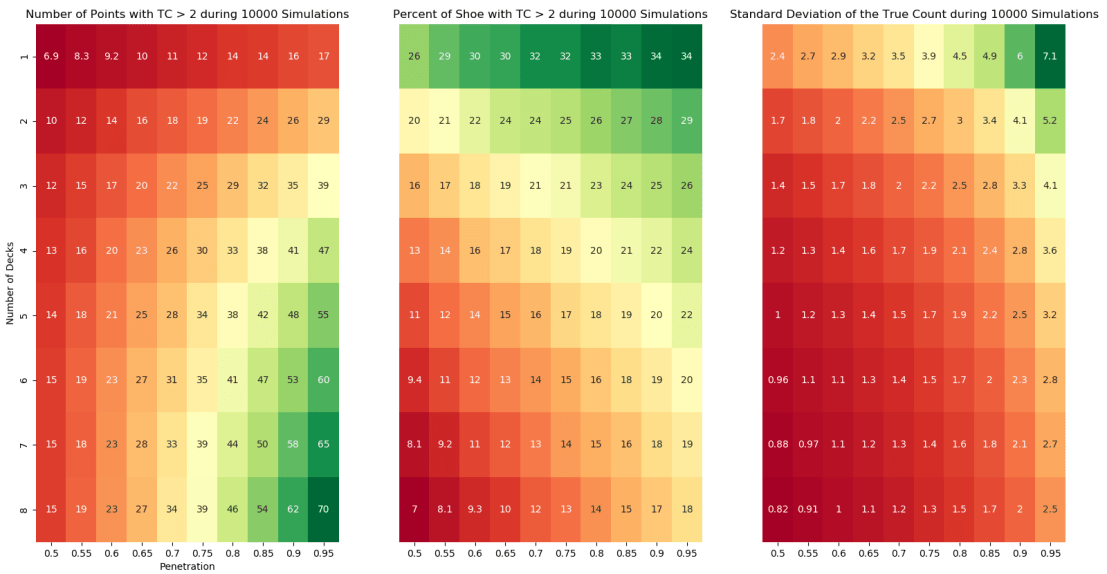
Figure 3: Heatmaps of Outcomes Based on Different Combinations of the Number of Decks and Depth of Penetration

These findings are consistent with previous analysis of Blackjack. The player can expect to spend the most time with the advantage in games using fewer decks and deeper penetration. The value of this advantage time is also improved by a larger variance. The variance is more dependent on the depth of penetration than the number of decks, but both affect its value. If we look at a standard game available at many casinos of 6 decks with 65% penetration, the player will have the TC > 2 for 13% of the shoe on average with a TC standard deviation of 1.3. If we were to find a 2-deck game with 90% penetration, the player will have the TC > 2 for 28% of the shoe on average with a TC standard deviation of 4.1. If these games have the same rules, the player will gain more of an edge with fewer decks and deeper penetration.

The code for generating this analysis can be found on Github here. An interesting topic to explore next would if the path that the TC takes when reverting back to zero affects expected value and if so, how?

Acknowledgements: Thank you to James Sweetman for helping me better understand the Blackjack concepts.

Constructing Continuous Futures Price Series

Welcome! If you enjoy these posts, please follow this blog via email and check out my Twitter feed located on the sidebar.

All of my previous analysis has focused on US equities, but today we begin the journey into another asset class, futures. Futures are traded via contracts where two parties agree to exchange a quantity of an asset for a price decided today and delivered at a specified date in the future. The expiration dates of the contracts vary based on the underlying asset and range from monthly to quarterly. To properly evaluate the profitability of trading strategies with historical futures contract data, it is necessary to combine these contracts into a continuous price series. This isn’t entirely straightforward because contango and backwardation factors cause contracts of the same underlying asset with different expiration dates to be priced differently. It is initially unclear how to best concatenate these price series, so I want to explore a few of the basic methods and their advantages. I’m interested in exploring futures strategies, so this was a necessary first step since Quandl’s free continuous futures data is of insufficient quality, but they provide high quality individual contract data. Becoming comfortable with the contract data while creating flexible, testable continuous price series is a valuable exercise. Additionally, I decided to use Python because I have not done a project with it and this is a useful applied problem to build some Python skills.

For this example, we will construct a variety of continuous price series for the commodity wheat. The first step is to pull the contract data from the Quandl API and store it appropriately (see the included code). To begin, let’s plot all the contracts’ prices to observe the behavior of the price data. As seen in Figure 1 below, although there is some consistency between the contracts, there is a significant amount of variance.

10.1 — Figure 1: Futures Prices of All Wheat Contracts

Ideally, to make this a backtest-ready series, we need to be trading a single contract at each point in time (or possibly a combination of contracts). The further we are from a contract’s expiration; the more price speculation is embedded into the price. The front or nearest month contract refers to the contract which has the soonest expiration date and thus has the least amount of speculation. Generally, front month contracts have the most trading activity, as measured by open interest. When expiration approaches, traders will roll their positions over to the next contract or let them expire. A basic approach to construct a continuous series would be to always use the front month contract’s price and when the current front month contract expires, switch to the new front month contract. There is one caveat, the price of the contracts when you rollover may not be the same, and in general, won’t be the same. These gaps will create artificial, untradeable price movements in the continuous series. To create a smooth transition between contracts, we can adjust them in such a way so that there won’t be a gap. We’ll refer to the size of this gap as the adjustment factor. Forward adjusting would shift the next contract to eliminate the gap by subtracting the adjustment factor from the next contract’s price series. Backward adjusting would shift the previous contract to eliminate the gap by adding the adjustment factor to the previous contract’s price series. Figure 2 below shows an example of these adjustments for an actual rollover.

Figure 2: Backward/Forward Adjusting Example

Now, when this approach is extended over multiple contracts the adjustment factors will simply cumulate so that prices for every contract are appropriately adjusted. The quality of the data is the same whether you backward or forward adjust. The difference is what needs to be recalculated with each new contract and what the values represent. The backward adjusted series’ current values represent the actual market values thus the historical data needs to be recalculated when a new contract is added to the series. The forward adjusted series does not require recalculating historical data but since each new contract that is added to the series needs to be adjusted, the new prices will not represent the actual market values. Figure 3 below shows the fully adjusted wheat series. Notice that the difference between the forward and backward adjusted series remains constant. This difference is the total adjustment factor.

10.3 — Figure 3: Expiration Adjusted Wheat Series

A point that becomes apparent, here, is that we are adjusting the price series, not the returns. The daily returns of the forward and backward adjusted series differ. When creating continuous prices, you are forced to choose between either correct P&L or correct returns. To adjust for correct returns, one would need to work with the daily log returns series of the contracts and then construct a usable price series from those. Dr. Ernest Chan’s second book covers this concept thoroughly on pg. 12-16.

Another approach to construct a continuous series is the perpetual method, which smooths the transitions between contracts by taking a weighted average of the contracts’ prices during the transition period. This can be weighted on time left to expiration, open interest, or other properties of the contracts. For this example, we will begin the transition to the next contract once its open interest becomes greater than the current contract and weight the prices during the transition based on open interest. As seen in Figure 4 below, this happens prior to the expiration of the contracts.

10.4 — Figure 4: 2014 Wheat Contracts’ Open Interest

Like the previous example, one could also forward/backward adjust using the open interest crossover date which is more realistic because of better liquidity. This option is available in the attached code. In our case, after this crossover date, we transition to the next contract over the next 5 days (the number of days is adjustable) based on open interest. Figure 5 below shows the slightly smoother perpetual adjusted series.

10.5 — Figure 5: Perpetual Adjusted Wheat Series

This smoothed price series may be advantageous for statistical research since it reduces noise in longer term signals but it contains prices that are not directly tradable. To trade the price during the transition period, one would have to rebalance their percentage of the current and next contract each day, which would incur transaction costs.

There are a variety of other adjustment methods, but the examples shown here provide a strong and sufficient foundation. A paper that I found very helpful and one that covers additional methods is available here. The Python code accompanying this post can be found here. I hope you found these examples helpful. In my next post, I am going to use these continuous series as I analyze futures trading strategies. Thanks for reading!